Hypothesis Tests Worked Examples (Business)

Worked Example - One Sample z-test

You work in the HR department at a large franchise and you are currently working in the expenses department. You want to test whether you have set your employee monthly allowances correctly. In the past it was believed that the average claim was $£500$ with a standard deviation of $150$, however you believe this may have increased due to inflation. You want to test if the monthly allowances should be increased. A random sample is taken of $40$ employees and gives a mean monthly claim of $£640$.

Perform a hypothesis test of whether you should increase your employees' monthly allowances.

Solution

This is a one sample $z$-test because you know the population standard deviation ($\sigma = 150$). It is also a One-tailed example because we are testing for an increase.

The hypotheses are:

$H_0: \mu = 500$

$H_1: \mu > 500$

Calculating the $z$-statistic using the formula above gives: $\dfrac{640 - 500}{\sqrt{\dfrac{150^2}{40}}} = 5.903$ (to 3 d.p)

Next, we look up this value in the $z$-table (see above). Since this is a one tailed example, we compare the values at the $z_{1- \alpha}$ level. At the $1\%$ level, you can see that $ 5.903 > 2.33$, so this is a significant result. This means we have sufficient evidence to reject the null hypothesis that there has been no change in the average employee expenses claim. Thus, you should increase the monthly allowances.

Worked Example - Paired Sample test

You want to examine how effective a computer course is for your employees and whether to require all of your employees to take the course. To decide whether the course is effective, you decide to enrol $10$ employees in the course and test them before and then again after the course. Their test scores are recorded below.

Has there been an improvement in test scores since taking the course?

Solution

This is a two sample paired t-test as we are testing the same sample twice. This is also a one tailed example as we have specified a direction (an increase in test scores). The mean of the differences is $\bar{d} = \dfrac{3-1+3+3+3+2+0+1+3+9}{10}=2.6$ and the corresponding sample standard deviation is $ s = 2.67$.

The null hypothesis is that the mean of the differences is zero and the alternative hypothesis is that the mean of the differences is greater than zero.

$H_0: \mu = 0$

$ H_1: \mu > 0$

The t-statistic is calculated using the formula $t = \dfrac{2.6}{\sqrt{\dfrac{2.67^2}{10}}} = 3.079$.

We now want to compare this value to the critical values on the t-table on $n-1 = 9$ degrees of freedom. We have a significant result as $3.079>2.821$ (circled in the table), so our t-statistic is significant at the $1\%$ level. This means we have sufficient evidence to reject the null hypothesis and we conclude that there is sufficient evidence to suggest that the course improves performance.

Here is a video tutorial showing how to solve this example using Minitab (ver. 16):

Worked Example - Two Sample Test

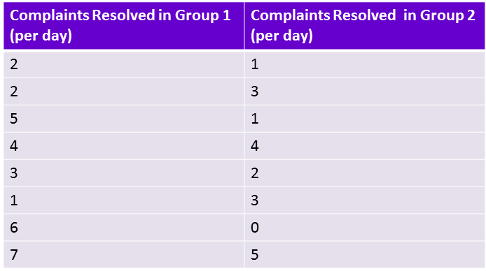
You are interested in the effect the workplace environment has on daily productivity. Your company deals with customer complaints. You decide to test how many complaints on average one group (group $1$) of advisors in a bright and light room where they are allowed to talk to colleagues handle in comparison to the average of another group (group $2$) who work in a plain windowless room with a strict no talking policy. Below is a table charting the number of complaints dealt with by each group.

Is there a difference in productivity between the two groups?

Solution

We need to use a two sample unrelated t-test, as we have two small samples with no relationship to one another (we have two different groups of people).

Firstly, set up the hypotheses:

$H_0: \bar{x}_1= \bar{x}_2 $

$H_1: \bar{x}_1\not = \bar{x}_2 $

The null hypothesis is that there is no difference in the means of the two groups and the alternative hypothesis is that there is a difference in the means (two-tailed example).

The mean resolved complaints for group $1$ is $\bar{x}_1 = 3.75$ and sample standard deviation $s_1 = 2.121$ ( to 3 d.p.) The mean resolved complaints for group $2$ is $\bar{x} = 2.375$ and sample standard deviation $s_2 = 1.685$ (to 3 d.p.)

Now we need to calculate the pooled standard deviation $s$ by inputting the above values into the formula: $s =\sqrt{\dfrac{(n_1 - 1)s_1^2 + (n_2 - 1)s_2^2}{n_1 +n_2 -2}}$ :

$ s = \sqrt{\dfrac{(7 \times 2.121^2) + (7 \times 1.685^2)}{14}} = 1.915$ (to 3 d.p.)

Now calculate the t statistic using the formula $ t = \dfrac{1.375}{\sqrt{1.916^2 \times \bigg(\dfrac{1}{8} + \dfrac{1}{8}\bigg)}} = 1.435$ (to 3 d.p.)

We need to compare this value to the critical values on the t-table (below) on $n_1+n_2 -2 = 14$ degrees of freedom. As you can see our t-statistic of $1.435$ is smaller than all of the critical values on $14$ degrees of freedom, so we can conclude that this is significant so we must reject the null hypothesis that the means are the same. The environment does affect work productivity.

Watch the following video for how to solve this example in Minitab (ver. 16):

Test Yourself

Try our Numbas test on hypothesis testing: Hypothesis testing and confidence intervals and also two-sample tests.

See Also

For more information about the topics covered here see hypothesis testing.