Normal Distribution (Business)
Normal Distribution
The Normal distribution is the most widely used and frequently occurring continuous probability distribution.
The formula for the pdf of the Normal distribution is:
\begin{equation} f(x) = \dfrac{1}{\sqrt{2\pi \times \sigma^2}} \mathrm{exp}\left(-\dfrac{{(x - \mu)}^2}{2\sigma^2}\right) \end{equation}
where $\mu$, the mean and $\sigma^2$ is the variance (the square of the standard deviation, $\sigma$)
If a random variable $X$ follows a Normal distribution we write $X$~$\mathrm{N}(\mu, \sigma^2)$
Illustrative Example
Suppose that the owner of a company selling climbing equipment already sells climbing helmets for children but wants to start selling helmets for adults as well.The company plans to sell separate helmets for men and for women and wants to know how many of each size (small, medium or large for male and female separately) to produce. The company may assume that a person's head size approximately follows a Normal distribution with a separate mean and variance for males and females So, using the Normal distribution as a model, the owner can order the appropriate numbers and sizes of helmets.
What does the Normal distribution look like?
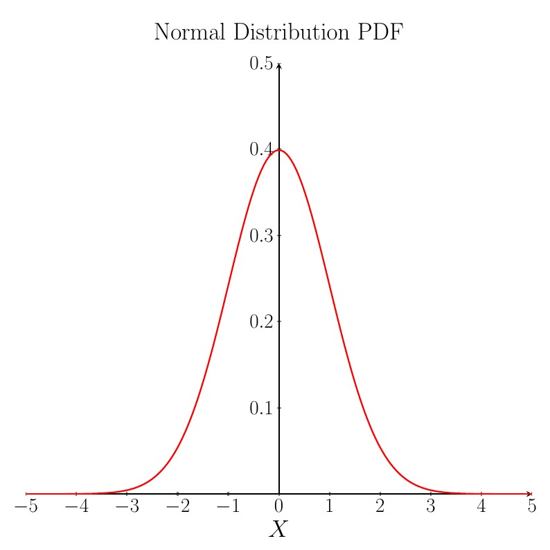
The probability density function (pdf) for a Normal random variable is bell-shaped and is symmetric about the mean value, $\mu$. In the plot below $\mu=0$. Although the plot only shows the curve in the range $-5 \leq X \leq +5$, the curve goes all the way out to minus infinity and plus infinity.
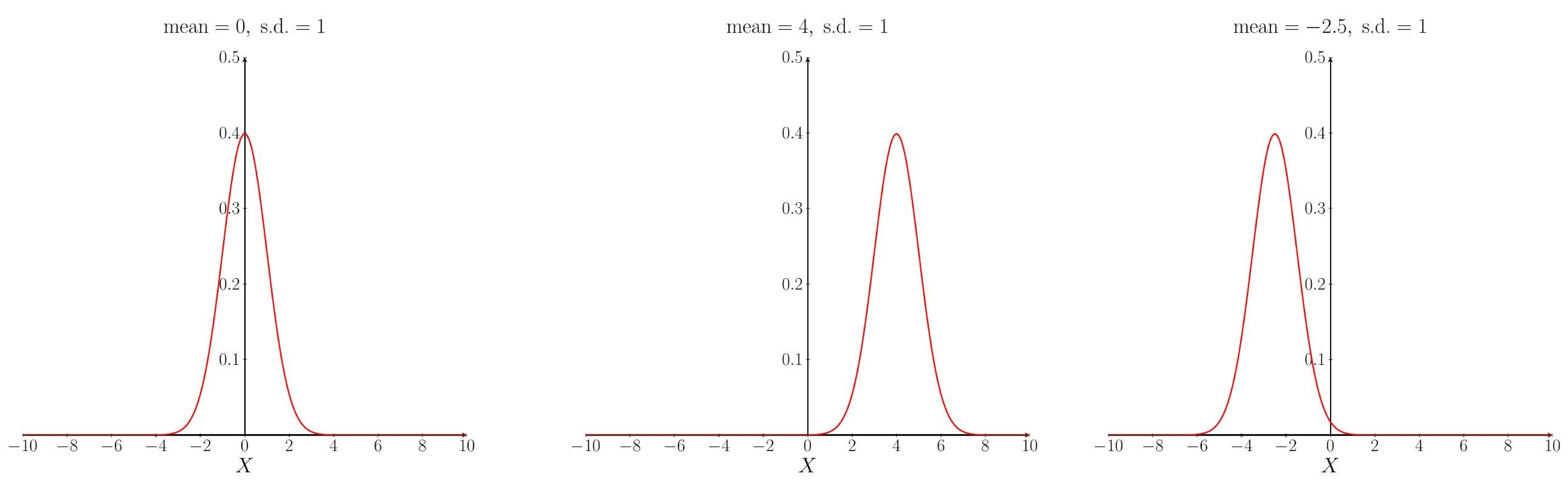
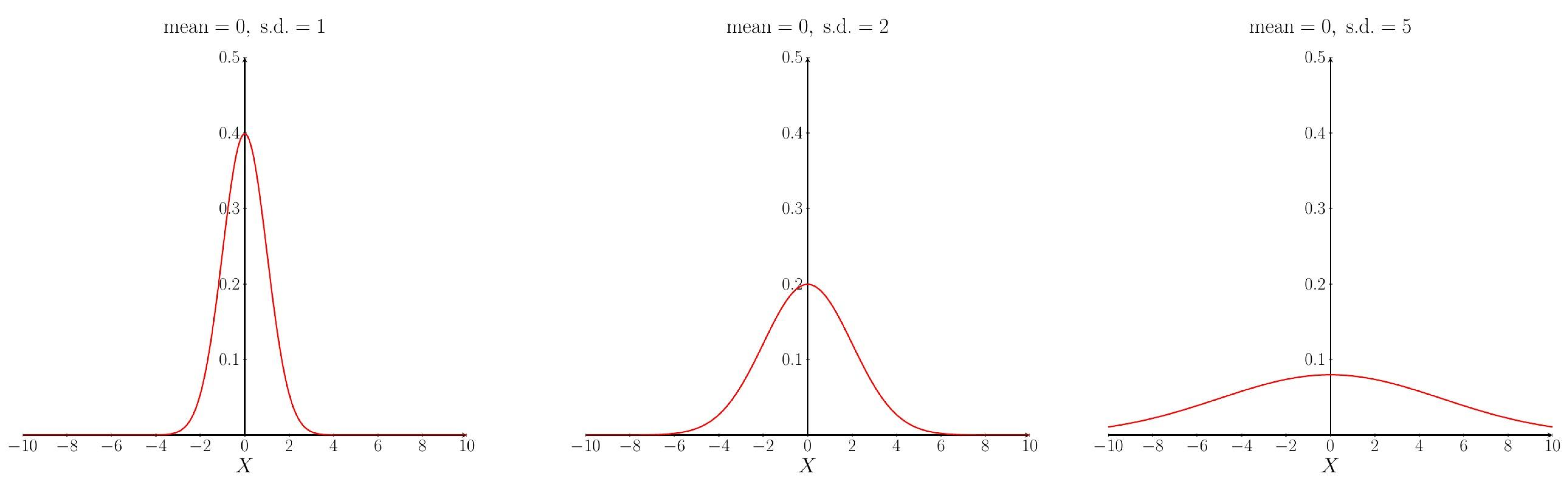
The shape of the pdf curve depends upon the values of the parameters $\mu$ and $\sigma$. Changing the mean $\mu$ affects the location (on the $X$-axis) of the peak of the curve: increasing the mean moves the curve to the right, decreasing the mean moves the curve to the left. The standard deviation $\sigma$ determines how spread out the curve is: increasing the standard deviation makes the curve more spread out and decreasing the standard deviation makes the curve narrower.
The effect of changing the mean.
The effect of changing the standard deviation.
Calculating Probabilities
Suppose we have a random variable $X$ which follows a Normal distribution with mean $0$ and standard deviation (s.d.) $1$.
$\mathrm{P}(0 \leq X \leq 1)$ is equal to the area of the shaded region on the graph shown below.
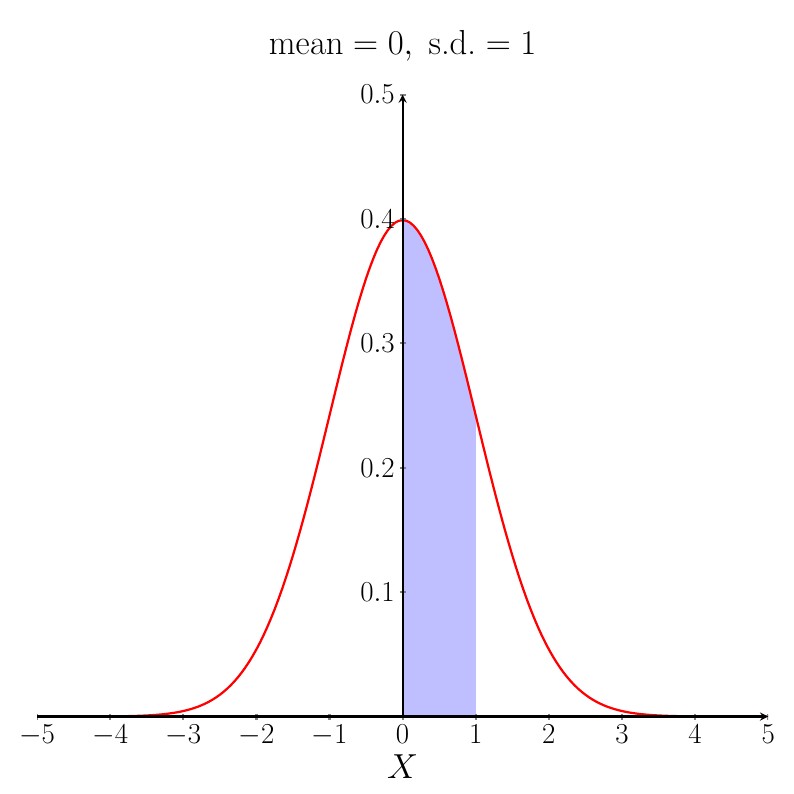
These probabilities are found by looking up standard Normal distribution tables or you can use computer packages, such as R and Minitab, to find them. For more detailed information about the Normal distribution, including how to look up probabilities in tables, click here. From the tables, we find that the shaded area above is equal to $0.3413$.
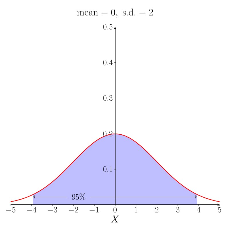
$95\%$ of the area under the Normal distribution $\mathrm{N}(\mu,\sigma^2)$ pdf curve lies in the range $\mu- 1.96 \times \sigma \leq X \leq \mu+ 1.96 \times \sigma$.
A good way to remember this is that $95\%$ of the area under the curve lies within roughly $2$ standard deviations of the mean. The figure below shows the case when the mean is $0$ and the s.d. is $2$.
Standardising
A Standard Normal distribution has $\mu = 0$ and $\sigma = 1$. A non-standard Normal random variable $X$, which has mean $\mu \neq 0$ and/or standard deviation $\sigma \neq 1$ can be standardised as follows:
Take $X$, the variable, and subtract its mean $\mu$, then divide by its standard deviation $\sigma$. We then call the result $Z$.
\begin{equation} Z = \dfrac{X-\mu}{\sigma}. \end{equation}
We then can compute probabilities using $Z$ and standard Normal tables.
Worked Example
Worked Example
The owner of Fredds, a chain of popular bakery stores in the North East, supplies all of her employees with a uniform. She is ordering a bundle of uniforms for new employees hired within the next year and needs to decide what sizes and how many uniforms of each size to buy. The only difference between uniforms is their height and the owner assumes that peoples' heights follow a Normal distribution with $\mu = 170$cm and $\sigma^2 = 49$cm. Calculate the probability that a randomly selected (future) employee is:
(A) Smaller than 160cm.
(B) Between 165cm and 175cm.
(C) Taller than 185cm.
Solution
Here, we have a Normal random variable, $X$~$\mathrm{N}(170,49)$. Firstly, we need to standardise $X$ to $Z$ where $\mu = 170$, $\sigma = \sqrt{49} = 7$. So, \begin{align} Z &= \dfrac{X-\mu}{\sigma}\\ &= \dfrac{X - 170}{7}\\ \end{align}.
'(A)
To find the probability that a randomly selected employee is smaller than 160cm, we first write: \begin{align} \mathrm{P}(X&<160).\\ \end{align}
Then standardise both sides of the inequality.
\begin{align} & \; \; \; \; \; \; \mathrm{P}\left (\dfrac{X - 170}{7} < \dfrac{160 - 170}{7} \right)\\ &\Rightarrow \mathrm{P} \left (Z< \dfrac{160 - 170}{7} \right)\\ &= \mathrm{P}(Z< -1.43)\;\;\text{ (to 2 d.p)}\\ \end{align}.
We then need to look up $Z=-1.43$ in a $Z$-table to find the corresponding probability.

|center
We find that the probability is $0.0764$. So, \begin{align} &\; \; \; \; \; \; \mathrm{P}(Z < -1.43) = 0.076 \text{ (to 3 d.p)}\\ &\Rightarrow \mathrm{P}(X< 160) = 0.076.\\ \end{align}
(B)
Now we require the probability that a randomly selected employee is taller than 165cm but smaller than 175cm. That is, we require
\begin{align} &\mathrm{P}(165

|center
From the table we can see that $\mathrm{P}(Z<2.14) = 0.984 \text{ (to 3 d.p)}$ so:
\begin{align} \mathrm{P}(X>185) &= 1 - 0.984\\ &=0.016 \text{ (to 3 d.p)}.\\ \end{align}
Test Yourself
Click on the following links to practise Numbas tests on the distributions on this page:
Test yourself: Numbas test on calculating probabilities from a normal distribution
Test yourself: Numbas test on the exponential distribution and uniform distribution