Numeracy, Maths and Statistics - Academic Skills Kit

Descriptive Statistics (Psychology)

ContentsToggle Main Menu 1 Introduction 2 Sampling 3 Measures of Location3.1 The Arithmetic Mean3.2 The Mode3.3 The Median 4 Measures of Spread4.1 The Range4.2 The Sample Variance $(s^2)$4.3 The Population Variance $(\sigma^2)$4.4 The Sample Standard Deviation $(s)$4.5 The Population Standard Deviation $(\sigma)$4.6 The Interquartile Range (IQR)4.7 The Standard Error (SE) of the Mean4.8 Notation in the above formulas explained: 5 Workbook 6 Test Yourself 7 See Also

Introduction

Given a dataset, your task may be to try to describe the main features of the data, or descriptive statistics, which could be influential in making decisions. For example, you may want to know how widely dispersed the data are about a central location; this will give you an idea of the variability of the dataset. You will have a choice of measures of central location and variability, you choose the ones that give you the most information depending on the type of data you have and in relation to the decisions you want to make.

If all the dataset information is available to you and you have sufficient software to analyse it e.g. R, SPSS or Minitab, then your task is to put the information into the program and choose the appropriate descriptive statistics.

However, the dataset information you want may not be fully available to you. This is particularly true for large populations where it is not feasible to extract all the data , e.g. for the the UK population; voting preferences, number of cars per household etc. In this case the usual method is to sample the population.

Sampling

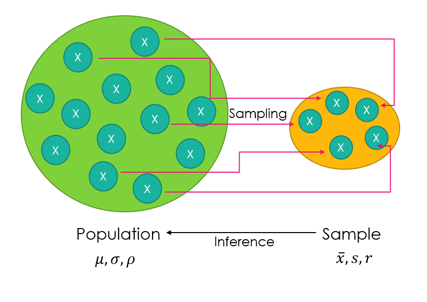
Sampling involves taking a small amount, or sample, of the entire population to draw conclusions and test hypotheses. For example, if you wanted to answer the question, “How many hours after school do children do homework in England?” it would be almost impossible and very time consuming to question every child in the country, so you instead take a sample of the population and test them, to make inferences about the overall population. There are different types of sampling: random and non-random, which both have advantages and disadvantages. For more information on this, see sampling.

Measures of Location

The following are ways of representing a representative value of the set of data.

The Arithmetic Mean

This is calculated by summing all of the data values and dividing by the total number of data items you have. It is normally called the mean or the average. If you have a data consisting of $n$ observations $(x_1,...,x_n)$ then the mean $(\bar{x})$ is given by the formula:

\begin{equation} \bar {x} = \frac{1}{n}\sum\limits_{i=1}^{n}\ x_i. \end{equation}

A sample mean is the mean of a sample taken from the population you are considering.
The population mean, often denoted by $\mu$, is the mean for the entire population you are studying. Often you do not know the population mean and have to estimate it from a sample mean.

The Mode

The mode is the most frequently occurring value in the data set. For instance in the set of data $3,4,4,5,4,6,7,8$ the modal value of the set is $4$, as $4$ occurs most frequently.

The Median

The median can be viewed as the middle value for a set of numeric data. To calculate this value, order the data values by increasing size:

For an odd number of points the median is the value that is in the middle i.e. for $n$ observations the middle number is the $\bigg(\dfrac{n+1}{2}\bigg)^\text{th}$term. For example, in the ordered set $1,3,4,4,5,6,7,7,8$ the median is the fifth number in this set which is $5$.

If you have an even number ($n$) of observations then there is no one middle number so you average the middle two values i.e. $\big(\frac{n}{2}\big)^\text{th}$ and $\big( \frac{n}{2} +1\big)^\text{th}$ values.

For example in the ordered set $10,13,14,14,16,17,17,17,18,19$, the median is the average of the middle two numbers; the fifth, $16$ and the sixth, $17$. Hence the median is $\dfrac{16 + 17}{2} = 16.5$.

See Mean, median and mode and Weighted averages for more information and more complex examples.

Measures of Spread

The Range

For a numeric dataset the range measures the difference between the greatest and least values.

We calculate this using the formula:

\begin{equation} \text{Range} =\text{Greatest value}- \text{ least value}. \end{equation}

The Sample Variance $(s^2)$

Is the square of the sample standard deviation. and measures the spread of the sample data values about the sample mean. The formula for the sample variance is therefore:

\begin{equation} s^2 = \frac{1}{n-1}\sum\limits_{i=1}^n(x_i - \bar {x})^2. \end{equation}

The Population Variance $(\sigma^2)$

The population variance measures the spread of the whole population. Note carefully that the population variance differs from the sample variance in that instead of dividing by $n-1$ we divide by $n$ so the formula becomes:

\begin{equation} \sigma^2 = \frac{1}{n}\sum\limits_{i=1}^n(x_i - \bar {x})^2. \end{equation}

The Sample Standard Deviation $(s)$

If we have taken a sample from a population, the sample standard deviation (SD) measures by how much the sample data deviates from the sample mean. The standard deviation is the positive square root of the variance. It is calculated using the formula:

\begin{equation} s = \sqrt{\frac{1}{n-1}\sum\limits_{i=1}^n(x_i - \bar {x})^2}. \end{equation}

The Population Standard Deviation $(\sigma)$

The population standard deviation (SD) measures by how much the population data deviates from the mean of the whole population. The formula is slightly different from that of the sample standard deviation.

\begin{equation} \sigma = \sqrt{\frac{1}{n}\sum\limits_{i=1}^n(x_i - \bar {x})^2}. \end{equation}

The Interquartile Range (IQR)

The IQR measures the range of the middle half of the data, and so is less affected by extreme observations. It is given by $Q3 - Q1$, where:

\begin{equation} \begin{split} &&Q1 = \frac{(n+1)}{4}^\text{th} \text{ smallest observation} \\&& Q3 = \frac{3(n+1)}{4}^\text{th} \text {smallest observation}. \end{split} \end{equation}

The Standard Error (SE) of the Mean

The sample mean is an estimator of the population mean. If we keep on taking samples and then obtain a dataset comprising these sample means, then the standard error is a measure of the spread of the sample means from the population mean. It is calculated using the following formula:

\begin{equation} \text{Standard Error (SE)} = \frac{\sigma}{\sqrt{n}}. \end{equation}

Note that of we take large samples,i.e. increase $n$, then the standard error of the mean becomes smaller.

For more information see Variance and standard deviation

Notation in the above formulas explained:

\begin{equation} \begin{split} \bar{x}&& = \text{Arithmetic mean} \\ x &&= \text {Individual data value} \\ s&& = \text{ Sample standard deviation} \\ \sigma &&= \text{ Population standard deviation} \\ s^2&&= \text{ Sample variance} \\ \sigma^2&&= \text{ Population variance} \\ n &&= \text{Sample size} \\ \sum \limits_{i=1}^n{x_i}&& = \text{Sum of of the data values} (x_1,\ldots,x_n). \end{split} \end{equation}

Workbook

This workbook produced by HELM is a good revision aid, containing key points for revision and many worked examples.

Descriptive statistics including work on measures of location.

Test Yourself

Try testing yourself on descriptive statistics.

You can also take this test on identifying parts of statistical formulas.