Chi-square Tests (Business)
Chi-Square Tests
There are two important applications of Chi-Square tests ($\chi^2$ tests) :
- Goodness-of-fit tests. We use $\chi^2$ tests to test the goodness of fit of data to a hypothetical pattern, for example, does the number of customers arriving at a fairground ride follow a Poisson distribution?
- Test for Association/Independence. For example, is there an association between the ratings by students of their course lecturers and the average exam mark on the courses? This involves qualitative data; the categories that lecturers fall into given by their student rating. The null hypothesis is that there is no association and the $\chi^2$ test examines this hypothesis.
There are rules to follow when using a $\chi^2$ test, listed below.
- No category has a mean of less than $5$.
- The categories should be as natural as possible.
- Keep to the raw data.
- Avoid categories that vastly exceed others.
Goodness-of-fit Tests
The Method
To carry out the test by hand the steps are as follows:
- Firstly, we need to identify the null and alternative hypotheses $H_0$ and $H_1$. For example, if we think our data might follow a Uniform distribution, then we would have:
\begin{align} H_0&: \text{Our data follows a Uniform distribution versus}\\ H_1&: \text{Our data does }\textbf{not }\text{follow a Uniform distribution.}\\ \end{align} Note: The Uniform distribution can be replaced with any other probability distribution.
- After collecting data, we calculate the Chi-Square statistic/value:
\begin{equation} \chi^2 = \sum {\frac{(O-E)^2}{E}} \end{equation}
where:
\begin{split} \\ O &&= \text{Observed frequencies} \\ E &&= \text{Expected frequencies} \\ \sum{}&& =\text{ Sum Of} \end{split}
- We then compare this statistic to a $\chi^2$ table on the appropriate degrees of freedom...
\begin{equation} \nu = (\text{number of categories after pooling}) - 1. \end{equation}
- Finally, we make our conclusion. If the Chi-Square value does not exceed the critical value (e.g. $p = 0.05$) then the null hypothesis will be accepted i.e. the data does follow the hypothetical pattern. If it does exceed the critical value, the null hypothesis must be rejected.
Worked Example 1
Worked Example - Chi-squared Goodness-of-fit Test
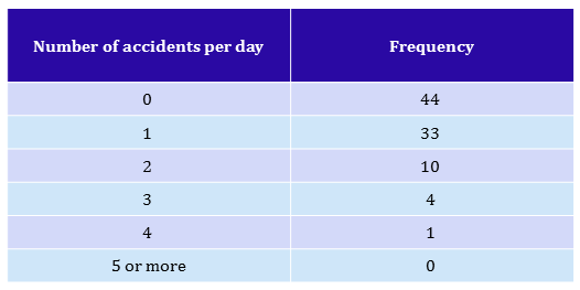
The number of accidents per day at a chocolate factory was recorded over the period of three months; the results are shown in the table below.
|center
Suggest a distribution that might fit these data, and test to see whether it is appropriate or not.
Solution
Since we are looking at the number of accidents in a certain time interval (day) and there is no fixed limit to the number of accidents which could happen, an appropriate distribution would be the Poisson distribution.
To see if the Poisson distribution is consistent with our data, we shall test the null hypothesis:
$H_0$: The number of accidents follow a Poisson distribution
versus the alternative:
$H_1$: The number of accidents does not follow a Poisson distribution.
To calculate our test statistic, we need to calculate our expected values/frequencies based on the Poisson distribution. We use the formula: \begin{equation} \mathrm{P}(X = r) = \dfrac{~\lambda^r \times e^{-\lambda}~}{r!} \end{equation}
to find the expected probabilities, and then multiply these by the total sample size $(92)$ to obtain the corresponding expected frequencies. Before we can use this formula, we need an estimate for $\lambda$. For the Poisson distribution, $\lambda$ is equal to the mean. Thus, we have:
\begin{align} \lambda &= \dfrac{(0 \times 44) + (1 \times 33) + (2 \times 10) + (3 \times 4) + (4 \times 1) + (5 \times 0)}{92}\\ &=0.75\\ \end{align}.
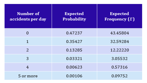
We now have $\lambda$ we can calculate the expected probabilities:
\begin{align} \mathrm{P}(X = 0) &= \dfrac{~0.75^0 \times e^{-0.75}~}{0!}\\ &= \dfrac{0.47237}{1}\\ &= 0.47237 \text{(5 d.p.)}.\\ &\\ \mathrm{P}(X = 1) &= \dfrac{~0.75^1 \times e^{-0.75}~}{1!}\\ &= \dfrac{0.75 \times 0.47237}{1}\\ &= 0.35427 \text{(5 d.p.)}.\\ &\\ \mathrm{P}(X = 2) &= \dfrac{~0.75^2 \times e^{-0.75}~}{2!}\\ &= \dfrac{0.5625 \times 0.47237}{2}\\ &= 0.13285 \text{(5 d.p.)}.\\ &\\ \end{align}
\begin{align} \mathrm{P}(X = 3) &= \dfrac{~0.75^3 \times e^{-0.75}~}{3!}\\ &= \dfrac{0.42188 \times 0.47237}{6}\\ &= 0.03321 \text{(5 d.p.)}.\\ &\\ \end{align}
\begin{align} \mathrm{P}(X = 4) &= \dfrac{~0.75^4 \times e^{-0.75}~}{4!}\\ &= \dfrac{0.31641 \times 0.47237}{24}\\ &= 0.00623 \text{(5 d.p.)}.\\ \end{align}
For the $5$ or more category, we can just add up all the other probabilities and subtract from $1$, since the entire probability distribution should sum to $1$. So we have
\begin{align} \mathrm{P}(X \geq 5) &= 1 - (0.47237 + 0.35427 + 0.13285 + 0.03321 + 0.00623)\\ &= 1 - 0.99894\\ &= 0.00106 \text{(5 d.p.)}.\\ \end{align}.
Thus, the expected frequencies can be found by multiplying the expected probabilities by the total sample size $(92)$ and then we can arrange them into a table:
|center
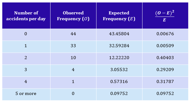
We can now calculate our test statistic.
|center
\begin{align} \chi^2 &= \sum{\dfrac{(O - E)^2}{E}~}\\ &= 0.00676 + 0.00509 + 0.40403 + 0.29209 + 0.31787 + 0.31787 + 0.09752\\ &=1.12336.\\ \end{align}
We now need to compare our test statistic to a value from a $\chi^2$ table. The degrees of freedom are (number of categories) - (number of parameters estimated) - $1 = 6 - 1 - 1 = 4$.
Thus, we use the following critical values:

|center
Since $1.12336 < 7.779$, the critical value at the $10$% significance level, there is no evidence against the null hypothesis $H_0$ so we cannot reject it. The number of accidents recorded per day at the chocolate factory follows a Poisson distribution.
Watch the following video for how to perform the Chi-Squared Goodness-of-fit test in Minitab (ver. 16):
Test for Association/Independence
Chi-Square tests can also be used to test for the association between attributes/independence (using Contingency Tables), for example, is there an association between the ability to drive and the distance commuted to work?
The Method
- You will need to use a $\chi^2$ test of independence when the data is given in the form of a contingency table.
- The method is very similar to the goodness-of-fit test.
- First, we form our hypotheses. Regardless of what the categorical variables are, if you are testing to see whether they are independent or not (associated) the hypotheses are:
\begin{align} H_0&: \text{There is no association between the categorical variables versus}\\ H_1&: \text{There }\textit{is}\text{ an association between the categorical variables.}\\ \end{align}
- Then we calculate the test statistic, which is the same as for the goodness-of-fit test.
\begin{equation} \chi^2 = \sum {\frac{(O-E)^2}{E}} \end{equation}
where:
\begin{split} \\ O &&= \text{Observed frequencies} \\ E&& = \text{Expected frequencies} \\ \sum{}&& =\text{ Sum Of} \end{split}
For this test, we need not worry about any probability distributions as we are just testing for independence. We can get our expected frequencies by using the following formula:
\begin{equation} E = \; \dfrac{\text{row total} \times \text{column total}}{\text{overall sample size}} \end{equation}
for each cell in the contingency table.
- Once we have the test statistic, we can find a $p$-value/critical value. The appropriate degrees of freedom to use is given by:
\begin{equation} \nu = (\text{number of rows }- 1) \times (\text{number of columns} - 1) \end{equation}
- Finally we form a conclusion. If the test statistics is greater than the critical value, we reject $H_0$ in favour of $H_1$. This is equivalent to saying there is sufficient evidence to suggest that the categorical variables are associated, or are not independent. Otherwise, we accept $H_0$.
Worked Example 2
Worked Example - Chi-squared test for Association/Independence
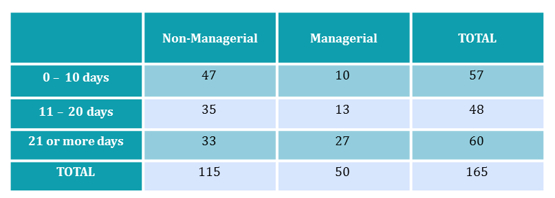
The following table includes data on the number of days sick leave taken by managerial and non-managerial employees of the department store, James Lewis, in the past year.
Is there an association between type of employee and number of days sick leave?
|center
Solution
Our hypotheses are: \begin{align} H_0&: \text{There is no association between type of employee and number of days sick leave.}\\ H_1&: \text{There is an association between type of employee and number of days sick leave.}\\ \end{align}
We need to calculate the expected frequencies before we can calculate the test statistic.
\begin{align} E_1 &= \; \dfrac{~\text{row total for '0 - 10 days'} \times \text{column total for 'Non-Managerial'}~}{~\text{total number of employees}~}\\ &= \dfrac{57\times115}{165}\\ &= 39.7273 \text{ (4 d.p.)}.\\ &\\ E_2 &= \; \dfrac{~\text{row total for '0 - 10 days'} \times \text{column total for 'Managerial'}~}{~\text{total number of employees}~}\\ &= \dfrac{57\times50}{165}\\ &= 17.2727 \text{ (4 d.p.)}.\\ &\\ E_3 &= \; \dfrac{~\text{row total for '11 - 20 days'} \times \text{column total for 'Non-Managerial'}~}{~\text{total number of employees}~}\\ &= \dfrac{48\times115}{165}\\ &= 33.4545 \text{ (4 d.p.)}.\\ &\\ E_4 &= \; \dfrac{~\text{row total for '11 - 20 days'} \times \text{column total for 'Managerial'}~}{~\text{total number of employees}~}\\ &= \dfrac{48\times50}{165}\\ &= 14.5455\text{ (4 d.p.)}.\\ &\\ E_5 &= \; \dfrac{~\text{row total for '21 or more days'} \times \text{column total for 'Non-Managerial'}~}{~\text{total number of employees}~}\\ &= \dfrac{60\times115}{165}\\ &= 41.8182 \text{ (4 d.p.)}.\\ &\\ E_6 &= \; \dfrac{~\text{row total for '21 or more days'} \times \text{column total for 'Managerial'}~}{~\text{total number of employees}~}\\ &= \dfrac{60\times50}{165}\\ &= 18.1818 \text{ (4 d.p.)}.\\ \end{align}
For convenience we shall arrange the data into a new table to calculate the test statistic.
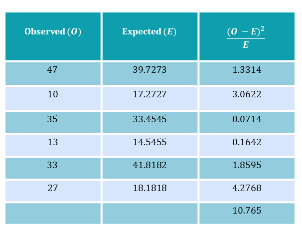
| center
Thus our test statistic is $\chi^2 = 11.0181$.
We need to compare this to critical values on $(3 - 1) \times (2 -1) = 2$ degrees of freedom.

|center
Since $10.765 > 9.210$ (the critical value at the $1\%$ level), we can conclude there is very significant evidence that there is an association between number of days sick leave and type of employee. We accept $H_1$.
Watch the following video to see how to perform the test in Minitab (ver. 16):
Test Yourself
Try our Numbas test on hypothesis testing: Hypothesis testing and confidence intervals and also two-sample tests.
See Also
For more information about the topics covered here see hypothesis testing.