Discrete Probability Models (Business)

This is a subject-specific page for Business 2 students.

What is a Discrete Probability distribution?

The probability distribution of a discrete random variable $X$ is the set $S$ of all the possible outcomes $X$ can take and corresponding probabilities $\mathrm{P}(x)$ (or equivalently $\mathrm{P}(X=x)$) for each $x \in S$ (each value of $x$ in the set $S$). Remember, for a discrete probability distribution to be valid, the probabilities must sum to one.

Business Example

Suppose that exactly 4 loan applications are reviewed each day by a small bank branch. Suppose further that these loans are accepted independently of each other so the probability that one of the four loans reviewed in a given day is accepted does not affect the probability that one of the other four loans is accepted. We have the following probabilities:

• No applications are accepted with probability $0.2$,
• $1$ application is accepted with probability $0.25$
• $2$ applications are accepted with probability $0.3$,
• $3$ applications are accepted with probability $0.15$ and
• $4$ are accepted with probability $0.1$.

This is an example of a discrete probability distribution and is valid because the probabilities sum to 1 ($0.2+0.25+0.3+0.15+0.1=1$). We can present this probability distribution as a table:

Cumulative Probabilities

If $X$ is a random variable then the cumulative probability ($\mathrm{P}(X \leq 4)$ for example) is the probability that $X$ takes any value less than or equal to 4.

If $X$ is a discrete random variable taking only positive values, then we can obtain this cumulative probability by summing each of the probabilities $\mathrm{P}(X=j)$ for $j=0, 1, 2, 3.$. That is,

\[\mathrm{P}(X \leq 4)=\mathrm{P}(X=0)+\mathrm{P}(X=1)+\mathrm{P}(X=2)+\mathrm{P}(X=3).\] Note: Since the sum of all of the probabilities must be 1, we have for any value $j$:

\[\mathrm{P}(X \leq j)=1-\mathrm{P}(X \gt j).\]

Thus if $\mathrm{P}(X \leq j)$ is more straightforward to calculate than $\mathrm{P}(X \gt j)$ (or vice versa), we can use the above fact to obtain one from the other. We will see examples of this below.

The Expectation and Variance

The expectation $\mathrm{E}[X]$ of a discrete random variable $X$ is the sum of each of the possible outcomes multiplied by their associated probabilities.

The variance $\mathrm{Var}(X)$ of a discrete random variable $X$ is defined as:

However it can be simplified to this expression:

where $\mathrm{E}[X^2]$ is the sum of each outcome squared and multiplied by its corresponding probability:

\[\sum\limits_{x \in S}{x^2 \times \mathrm{P}(x)}\]

and $\mathrm{E}[X]^2$ is the mean, $\mathrm{E}[X]$, squared:

\[\left(\sum\limits_{x \in S}{x \times \mathrm{P}(x)}\right)^2\].

Note: We also denote $\mathrm{E}[X]$ as $\mu$.

Example 1

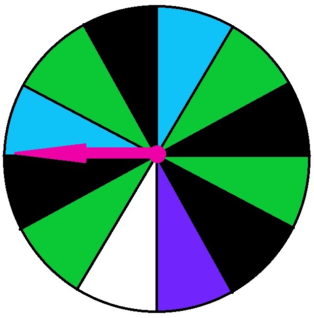
In a game, there is a spinner with twelve equally sized segments. There are four green segments, two blue segments, one purple segment, one white segment and four black segments. If a player spins:

• green, they must move forward $2$ spaces;
• blue, they must move forward $1$ space;
• purple, they must move forward $3$ spaces;
• white, they move back $1$ space and
• black, they do not move.

(A) What is the expected number of spaces a player will move in a turn?

(B) What is the variance of the number of spaces moved?

Solution (A)

Firstly, we can think of each colour as a number: a positive number represents moving forwards in the game and a negative number represents moving backwards.

Now we need to calculate the associated probabilities for these values.

Let $X$ denote the number of spaces moved.

\begin{align} \mathrm{P}(X = 2) &= \dfrac{\text{Number of Green Segments}}{\text{Total Number of Segments}}\\ &=\dfrac{4}{12}\\ &=\dfrac{1}{3}\\ \end{align}

\begin{align} \mathrm{P}(X = 1) &= \dfrac{\text{Number of Blue Segments}}{\text{Total Number of Segments}}\\ &=\dfrac{2}{12}\\ &=\dfrac{1}{6}\\ \end{align}

\begin{align} \mathrm{P}(X = 3) &= \dfrac{\text{Number of Purple Segments}}{\text{Total Number of Segments}}\\ &=\dfrac{1}{12}\\ \end{align}

\begin{align} \mathrm{P}(X = -1) &= \dfrac{\text{Number of White Segments}}{\text{Total Number of Segments}}\\ &=\dfrac{1}{12}\\ \end{align}

\begin{align} \mathrm{P}(X = 0) &= \dfrac{\text{Number of Black Segments}}{\text{Total Number of Segments}}\\ &=\dfrac{4}{12}\\ &=\dfrac{1}{3}\\ \end{align}

Now we can put these values into a table.

Now we can see that we have a discrete probability distributions and the distribution is valid as the probabilities sum to one.

To calculate the expectation we use the above formula, $\mathrm{E}[X] = \sum\limits_{x \in S}{x \times P(X = x)}$ as follows:

\begin{align} \mathrm{E}[X] &= 2 \times \dfrac{1}{3} + 1 \times \dfrac{1}{6} + 3 \times \dfrac{1}{12} + (-1) \times \dfrac{1}{12} + 0 \times \dfrac{1}{3}\\ &= \dfrac{2}{3} + \dfrac{1}{6} + \dfrac{1}{4} - \dfrac{1}{12} + 0\\ &= 1\\ \end{align}

So the expected number of spaces moved in one turn is $\mathrm{E}[X]=1$.

Solution (B)

To calculate the variance we use the formula: $\mathrm{Var}(X) = \mathrm{E}[X^2] - (\mathrm{E}[X])^2$.

First we need to square each value of $x$ and multiply by the associated probabilities.

Thus: \begin{align} \mathrm{E}[X^2] &= 4 \times \dfrac{1}{3} + 1 \times \dfrac{1}{6} + 9 \times \dfrac{1}{12} + 1 \times \dfrac{1}{12} + 0 \times \dfrac{1}{3}\\ &= \dfrac{4}{3} + \dfrac{1}{6} + \dfrac{3}{4} + \dfrac{1}{12} + 0\\ &= \dfrac{7}{3}\\ \end{align}

From above we have $\mathrm{E}[X] = 1$, so $(\mathrm{E}[X])^2=1^2 = 1$.

The variance is thus:

\begin{align} \mathrm{Var}(X) &= \mathrm{E}[X^2] - (\mathrm{E}[X])^2\\ &=\dfrac{7}{3} - 1\\ &=\dfrac{4}{3}.\\ \end{align}

Combinations and Permutations

Combinations

A combination is a way of selecting a number of items from a collection of items where the order of selection is not important. Combinations can be used to calculate probabilities, which we shall demonstrate with an example.

Illustrative Example

Imagine you are about to be shipwrecked on a deserted island. There is some rope, a knife, a box of matches and a blanket, but you can only take two items with you before the ship sinks. How many different ways are there of choosing two items? The different ways of choosing two items are combinations (since order is not important) and are listed below:

1. Rope & knife
2. Rope & matches
3. Rope & blanket
4. Knife & matches
5. Knife & blanket
6. Matches & blanket.

So, there are six different ways of selecting two items.

Now imagine the items are all in unmarked identical wooden boxes, so you do not know which items you are selecting. What is the probability you have selected the knife and matches?

\begin{equation} \mathrm{P}(\text{select knife and matches}) = \dfrac{\text{Number of ways of selecting the knife and matches}}{\text{Total number of combinations}} =\dfrac{1}{6} \end{equation}

With this number of items, it is quite easy to list all the possible selections. However, for larger numbers of items listing all of the possible selections can become tedious and time consuming. Fortunately there is a much faster way of calculating such combinations. The formula is:

where $n!$ denotes the factorial of $n$ ($n!=n\times(n-1)\times(n-2)\times...\times1$), $n$ is the total number of items (e.g. people. numbers, objects...), $r$ is how many items we want to “choose” and $r \leq n$. We pronounce this formula as “$n$ C $r$” or “$n$ choose $r$”.

We can now use this formula to calculate how many ways there are of selecting six items from twelve as follows: \begin{align} {}^{12}\mathrm{C}_6 &=\dfrac{12!}{6!(12-6)!}\\ &=\dfrac{12\times11\times\times10\times9\times8\times7\times6\times5\times4\times3\times2\times1}{(6\times5\times4\times3\times2\times1)\times(6\times5\times4\times3\times2\times1)}\\ &=\dfrac{479001600}{720\times720}\\ &=924. \end{align}

Selecting lottery numbers is an example of choosing a combination. A person must pick $6$ numbers from $49$. With each draw there is only one winning combination. But how many combinations are possible?

There are ${}^{49}\mathrm{C}_6 = 13983816$ possible combinations or ways of picking $6$ numbers from the $49$ possible numbers where order doesn't matter. This means that the probability of winning the lottery is $\dfrac{1}{13983816}.$

Permutations

A permutation is a way of selecting a specified number of items from a collection of items where the order of selection is important. Another way of thinking about this is that it is a way of arranging a number of items.

We use the formula:

where $n!$ denotes the factorial of $n$ ($n!=n\times(n-1)\times(n-2)\times...\times1$), $n$ is the total number of items (e.g. people. numbers, objects...), $r$ is how many items we want to arrange from the $n$ items and $r \leq n$. where $n$ is the total number of things, $r$ is how many things we are choosing and $r \leq n$. As with combinations, we can also use permutations to help calculate probabilities.

Illustrative Example

Imagine you have been on the deserted island for some time. There are five survivors, including you. You decide to have a race as there is not much to do on the island. How many different outcomes are there for this race? How many different options are possible for first, second and third position?

Solution

Here we have a total of $5$ “items” (survivors). Each outcome of the race is a different arrangement or permutation of these 5 items so we can use the above formula:

\[{}^5\mathrm{P}_5 = 120\]. There are 120 different outcomes for this race.

The number of different options for the first three positions is an arrangement of $3$ items ($r$ in our formula) from a total of $5$ items ($n$ in the formula). There are thus:

\[{}^5\mathrm{P}_3 = 60\] different options for first, second and third position.

The Binomial Distribution

Let $X$ be the number of successes in an experiment/trial.

When the following statements are true:

• There are a fixed number of experiments/trials, $n$.
• There are only two possible outcomes for each trial, usually called 'success' or 'failure'.
• There probability of 'success' $p$ is constant (does not change for each trial). Note: the probability of failure will be $1 -p$.
• The outcome of each trial is independent of all other trials, i.e. what happens in one trial does not affect the outcome in another trial.

we say that $X$ “follows a Binomial Distribution” and we write $X\sim\mathrm{Bin}(n,p)$.

The probability of $r$ successes and $(n-r)$ failures can be calculated using the formula:

where $r$ can take the values $0,1,2,...n$.

Note:

• ${}^nC_r$ is just a combination.
• $X$ cannot be greater than $n$ ($X\leq n$) since there are only $n$ trials in total.

An example of the Binomial distribution in Business

At a chocolate factory in Slough with 120 production workers, there is a $10$% chance that a worker will be absent on any given day. The probability that one worker is assumed not to affect the probability that another is absent. The factory is able to operate on any given day as long as there are no more than 50 workers absent on that day. What is the probability that any $2$ out of $9$ randomly chosen workers will be absent next Monday?

Solution

This situation can be described by a Binomial Distribution since we have:

• a fixed number ($9$) of trials (workers).
• each trial has two possible outcomes, “success” (the worker is absent) or “failure” (the worker is not absent).
• the probability of success (0.1) is constant.
• the outcome of each trial is independent of the outcome of all other trials.

Let $X$ denote the number of absent workers. Using the above formula, the probability that $2$ out of $9$ randomly chosen workers will be absent is:

\begin{align} \mathrm{P}(X =2) &= {}^9\mathrm{C}_2 \times 0.1^2 \times(1-0.1)^{9-2}\\ &=36 \times 0.1^2 \times(0.9)^{7}\\ &=0.172 \text{ (to 3 d.p.).}\\ \end{align}

See Example 2, showing how to calculate binomial probabilities. The solution to this example can be found here.

Expectation and Variance of a Binomial Distribution

If $X\sim\mathrm{Bin}(n,p)$, then:

What does a Binomial Distribution look like?

Since the Binomial distribution is a discrete probability distribution we can represent it graphically as a bar chart. Below is a plot for the random variable $Y$ ~ $\mathrm{Bin}(10,0.5)$. The distribution is symmetric around $5$ as this is the mean of the distribution: $\mathrm{E}(Y)=n\times p=10\times 0.5=5$..

If we change the value of $p$ it skews the plots (makes them asymmetric) and if we increase the size of $n$ the barplot starts to represent a bell-shaped curve more. We can see this in the plots below.

Example 2

There are ten customers in a shop. The probability that an individual customer buys something is 0.4.

(A) Calculate the probability that one customer buys something.

(B) Calculate the probability that four customers buy something.

(C) Calculate the probability that at most two people buy something.

(D) What is the probability that at least two people buy something?

'''(E) How many customers do we expect to buy something?

Solutions

Let $Y$ denote the number of customers who buy something. Here $n = 10$ and $p = 0.4$. So we have $Y \sim \mathrm{Bin}(10,0.4)$

(A)

To calculate the probability that exactly one customer buys something we use the formula above in the first orange box for a Binomial probability with $n=10, p = 0.4 \text{ and } r = 1$: \begin{align} \mathrm{P}(Y = 1) &= {}^{10}\mathrm{C}_1 \times 0.4^{1} \times(1 - 0.4)^{10-1}\\ &={}^{10}\mathrm{C}_1 \times0.4\times0.6^{9}\\ &=0.040\text{ ( 3 d.p.)}.\\ \end{align}

(B)

Using the same formula as in part (A) we have: \begin{align} \mathrm{P}(Y = 4) &= {}^{10}\mathrm{C}_4 \times 0.4^{4} \times(1 - 0.4)^{10-4}\\ &={}^{10}\mathrm{C}_4 \times0.4^{4}\times0.6^{6}\\ &=0.251 \text{ (3 d.p.)}.\\ \end{align}

(C)

Here we are required to calculate the cumulative probability $\mathrm{P}(Y \leq 2)$. Summing the probabilities $\mathrm{P}(Y=j)$ for $j=0, 1, 2$, we have:

\begin{align} \mathrm{P}(Y \leq 2) &= \mathrm{P}(Y=0) \; + \; \mathrm{P}(Y=1) + \; \mathrm{P}(Y=2)\\ &= \big({}^{10}\mathrm{C}_0 \times 0.4^{0} \times(1 - 0.4)^{10-0}\big) + \big({}^{10}\mathrm{C}_1 \times 0.4^{1} \times(1 - 0.4)^{10-1}\big) + \big({}^{10}\mathrm{C}_2 \times 0.4^{2} \times(1 - 0.4)^{10-2}\big)\\ &= \big({}^{10}\mathrm{C}_0 \times0.4^{0}\times0.6^{10}\big) + \big({}^{10}\mathrm{C}_1 \times0.4^{1}\times0.6^{9}\big)+ \big({}^{10}\mathrm{C}_2 \times0.4^{2}\times0.6^{8}\big)\\ &=0.0060+0.0403+0.1209\\ &=0.167\text{ (3 d.p.)}.\\ \end{align}

Calculating the above probability, we needed to add up only three binomial probabilities. However, what if we had to calculate $\mathrm{P}(Y\leq7)$? We would have to calculate eight different probabilities and then add them up! Fortunately, there are published tables of the cumulative probabilities of the binomial distribution available that we can use for this purpose.

Alternatively we could have used the fact that, since $n=10$ for this distribution (so $X \leq 10$) and the sum of the probabilities must be 1,

\begin{align} \mathrm{P}(Y\leq7)&=1- \mathrm{P}(Y\gt7)\\ &= 1-(\mathrm{P}(Y=8) + \mathrm{P}(Y=9) + \mathrm{P}(Y=10))\\ \end{align}

(D)

Here we wish to calculate $\mathrm{P}(Y\geq2)$.

Rather than calculating $\mathrm{P}(Y=2)+\mathrm{P}(Y=3)+...+\mathrm{P}(Y=10)$, we can instead use the fact that $\mathrm{P}(Y\geq2)=1-\mathrm{P}(Y\lt2)$. We then only need to calculate $\mathrm{P}(Y\leq1)$ and subtract this from $1$ to obtain the probability $\mathrm{P}(Y\geq2)$.

\begin{align} \mathrm{P}(Y\geq2) &= 1-\mathrm{P}(Y\leq1)\\ &= 1 - \mathrm{P}(Y=1) - \mathrm{P}(Y=0)\\ &= 1 - \big({}^{10}\mathrm{C}_1 \times 0.4^{1} \times(1 - 0.4)^{10-1}\big) - \big({}^{10}\mathrm{C}_0 \times 0.4^{0} \times(1 - 0.4)^{10-0}\big)\\ &= 1 - 0.0403 - 0.0060\\ &= 0.954 \text{ (3 d.p.)}.\\ \end{align}

(E)

Using the expectation formula, we would expect $10 \times 0.4 = 4$ customers to buy something.

Note that the variance is $10 \times 0.4 \times(1-0.4) = 2.4$.

The Poisson Distribution

Now suppose the following hold:

• There is no natural upper limit to the number of trials.
• Events occur independently, at an average rate $\lambda$ ($\lambda$ is a Greek letter and is pronounced 'lamb-da') within a specified time interval

The Poisson distribution is a useful general model for count data. For example:

• The number of people entering a supermarket per hour.
• The number of Polish cavalry officers kicked by their horses each year.
• The number of cars passing a point on a road every minute.

Under these conditions, the probability that there are $r$ events observed within the interval has a Poisson Distribution and we write $X\sim\mathrm{Po}(\lambda)$.

The probability of r successes in a specified interval can be calculated using the formula:

Where $ e$ is the exponential function and $r!$ is $r$ factorial.

Expectation and Variance of the Poisson Distribution

If $X\sim\mathrm{Po}(\lambda)$ then the expectation and variance are given by:

An example of the Poisson distribution in Business

A company selling personalised T-shirts owns a website where customers can purchase T-shirts online at a price of £$15$ per T-shirt and a delivery charge of £$2.50$ per T-shirt to anywhere within the UK (the company does not currently ship its T-shirts outside of the UK). It is believed that on average $2$ orders arrive per minute. If the number of orders received in a minute exceeds $5$, then the website crashes, meaning the website becomes inaccessible to the public for ten minutes.

(A) What is the value of $\lambda$?

(B) Calculate the probability that the website crashes at between $10:30$am and $10:31$am tomorrow morning given that the website is accessible to the public at $10:30$am.

(C) Calculate the probability that the number of orders in any one-minute interval is the expected number of orders.

(D) What is the variance of the number of orders per minute?

Solution

The number of orders arriving at the website per minute is modelled by a $\mathrm{Poisson}(2)$ distribution (since we have an average of $2$ “successes” within a specified time limit.)

(A) Recall that for a Poisson distribution $\lambda$ is the expectation or average rate of successes (arrivals of orders). In this example we have been told that the average number of orders per minute is 2. We therefore have $\lambda = 2$.

(B) The probability that the website crashes between $10:30$am and $10:31$am morning is the same as the probability of the website crashing in any one minute interval.

Let $X$ denote the number of orders in a one-minute interval. We know that the website crashes if the number of orders exceeds 5 in one minute. We thus have:

$\mathrm{P}$(website crashes between $10:30$am and $10:31$am) $=\mathrm{P}(X \gt 5)$, where:

\begin{align} \mathrm{P}(X \gt 5) &=1-\mathrm{P}(X \leq 5)\\ &=1-(\mathrm{P}(X =0) + \mathrm{P}(X =1) + \mathrm{P}(X =2) + \mathrm{P}(X =3) + \mathrm{P}(X =4))\\ &=1-\left(\dfrac{2^0 \times e^{-2}}{0!} + \dfrac{2^1 \times e^{-2}}{1!} + \dfrac{2^2 \times e^{-2}}{2!} + \dfrac{2^3 \times e^{-2}}{3!} + \dfrac{2^4 \times e^{-2}}{4!}\right)\\ &=0.095 \text{ (to 3 d.p.)}.\\ \end{align}

Note: in this example we were able to sum the probabilities to obtain $\mathrm{P}(X \leq 5)$: i.e.

\[\mathrm{P}(X \leq 5)=\mathrm{P}(X =0) + \mathrm{P}(X =1) + \mathrm{P}(X =2) + \mathrm{P}(X =3) + \mathrm{P}(X =4)\]

because the Poisson is a discrete probability distribution.

(C) We have:

\begin{align} \mathrm{P}(X= \lambda)&=\mathrm{P}(X =2)\\ &=\dfrac{2^2 \times e^{-2}}{2!}\\ &=0.27 \text{ (to 2 d.p.)}. \end{align}

(D) Using the formula for the variance of a Poisson distribution we have:

\begin{align} \mathrm{Var(X)}&=\lambda\\ &=2. \end{align}

What does a Poisson distribution look like?

Below are bar plots of a $\mathrm{Poisson}(2)$ distribution and a $\mathrm{Poisson}(5)$ distribution.

Example 3

At a call centre the average number of calls received per minute is $7$.

Calculate the probability that, in the next minute, there are:

(A) four calls.

(B) eight calls.

(C) zero calls.

(D) at most three calls.

(E) What is the expected number of calls in a minute?

Solution

(A) Let $X$ denote the number of calls received by the call centre in a minute.

The number of calls received by the call centre per minute follows an average rate of $7$. Therefore $X\sim\mathrm{Po}(7)$ and so:

\begin{align} \mathrm{P}(X=4) &= \dfrac{7^4 \times e^{-7}}{4!}\\ &=0.091\text{(3 d.p.)}\\ \end{align}

(B) Now we need to calculate $\mathrm{P}(X=8)$.

\begin{align} \mathrm{P}(X=8) &= \dfrac{7^8 \times e^{-7}}{8!}\\ &=0.130\text{ (3 d.p.)}\\ \end{align}

(C) Now we need to calculate $\mathrm{P}(X=0)$. \begin{align} \mathrm{P}(X=0) &= \dfrac{7^0\times e^{-7}}{0!}\\ &=e^{-7}\\ &=0.001\text{ (3 d.p.)}\\ \end{align}

(D)

\begin{align} \mathrm{P}(X\leq3) &= \mathrm{P}(Y=0) + \mathrm{P}(Y=1) + \mathrm{P}(Y=2) + \mathrm{P}(Y=3)\\ &= \dfrac{7^0 \times e^{-7}}{0!} + \dfrac{7^1 \times e^{-7}}{1!} + \dfrac{7^2 \times e^{-7}}{2!} + \dfrac{7^3 \times e^{-7}}{3!}\\ &= 0.001+0.006+0.022+0.052\\ &= 0.082 \text{ (3 d.p.)}\\ \end{align}

(E) The expected number of calls per minute is the same as the rate for the Poisson Distribution, $7$.

Note: There are also Poisson tables available which can tell us the cumulative probabilities, which is useful for when $r$ is relatively large, for example, $P(X \leq 12)$.

Using the Poisson Distribution as an Approximation to the Binomial Distribution

When the value of $n$ is very large it can be very tedious and time-consuming to calculate probabilities using the Binomial distribution. However, for very large $n$ and very small $p$ the Poisson distribution can be used as an approximation to the Binomial distribution, where larger values of $n$ and smaller values of $p$ result in a better approximation.

The Poisson approximation to the Binomial distribution has mean $\lambda=np$ (where $n$ is the number of trials and $p$ is the probability of success for a Binomial distribution) and the same variance $\lambda=np$. Thus we have:

\begin{align} \mathrm{P}(X = r)& \cong \dfrac{(np)^r \times e^{-np}}{r!}, r = 0,1,...\\ \end{align}

Worked Example

Suppose in a small town there are $5000$ business and a fire occurs in any given business with probability $0.001$ over a decade. What's the probability that there is at most one fire in the next decade?

Solution

Let $X$ denote the number of fires in the city in the next decade. We wish to find $\mathrm{P}(X\leq1)$.

First we shall calculate this using the binomial distribution.

\begin{align} \mathrm{P}(X\leq1) &= \mathrm{P}(X = 0) + \mathrm{P}(X = 1)\\ &= {}^{5000}C_0 \times 0.001^{0} \times 0.999^{5000} + {}^{5000}C_1 \times 0.001^{1} \times 0.999^{4999}\\ &= 0.00672+0.03364\\ &= 0.040\text{ (3 d.p.)}\\ \end{align}

Now we calculate using the Poisson approximation to this Binomial distribution. Here, $\lambda = \mathrm{E}[X] = n \times p = 5000 \times 0.001 = 5$ so $X\sim\mathrm{Po}(5)$.

\begin{align} \mathrm{P}(X\leq1) &= \mathrm{P}(X=0) + \mathrm{P}(X=1)\\ &= \dfrac{5^0 e ^{-5}}{0!} + \dfrac{5^1 e ^{-5}}{1!}\\ &= 0.00674 + 0.03369\\ &= 0.040\text{ (3 d.p.)}. \end{align}

As we would expect, the two methods give the same result (to 3 d.p), which shows that in this instance the Poisson distribution is a good approximation to the Binomial distribution .

An insurance company could use this approximation to calculate how likely it is a business will need to claim for fire damage or the expected number of claims likely to be made.

Test Yourself

To practice questions on the Binomial distribution and Poisson distribution click the following link:

Numbas test.

See Also

For information on continuous probability distributions see here.