Coefficient of Determination, R-squared
Definition
The coefficient of determination, or $R^2$, is a measure that provides information about the goodness of fit of a model. In the context of regression it is a statistical measure of how well the regression line approximates the actual data. It is therefore important when a statistical model is used either to predict future outcomes or in the testing of hypotheses. There are a number of variants (see comment below); the one presented here is widely used
\begin{align} R^2&=1-\frac{\text{sum squared regression (SSR)}}{\text{total sum of squares (SST)}},\\ &=1-\frac{\sum({y_i}-\hat{y_i})^2}{\sum(y_i-\bar{y})^2}. \end{align} The sum squared regression is the sum of the residuals squared, and the total sum of squares is the sum of the distance the data is away from the mean all squared. As it is a percentage it will take values between $0$ and $1$.
Interpretation of the $R^2$ value
Here are a few examples of interpreting the $R^2$ value:
$R^2$ Values |
Interpretation |
Graph |
|---|---|---|
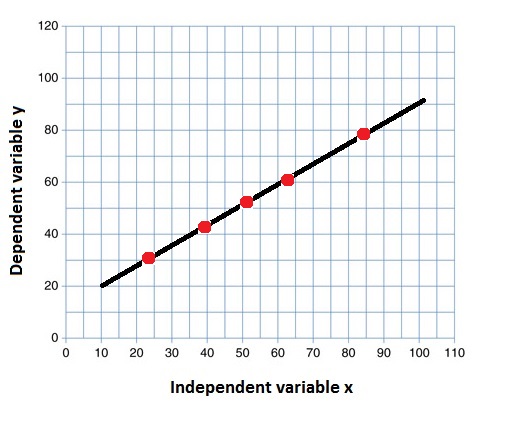
$R^2=1$ |
All the variation in the $y$ values is accounted for by the $x$ values |
|
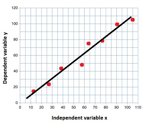
$R^2=0.83$ |
$83$% of the variation in the $y$ values is accounted for by the $x$ values |
|
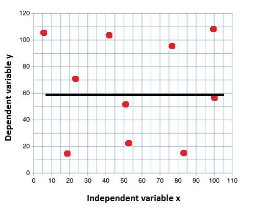
$R^2=0$ |
None of the variation in the $y$ values is accounted for by the $x$ values |
|
Worked Example
Worked Example
Below is a graph showing how the number lectures per day affects the number of hours spent at university per day. The equation of the regression line is drawn on the graph and it has equation $\hat{y}=0.143+1.229x$. Calculate $R^2$.

|text-top|400px
Solution
To calculate $R^2$ you need to find the sum of the residuals squared and the total sum of squares.
Start off by finding the residuals, which is the distance from regression line to each data point. Work out the predicted $y$ value by plugging in the corresponding $x$ value into the regression line equation.
- For the point $(2,2)$
\begin{align} \hat{y}&=0.143+1.229x\\ &=0.143+(1.229\times2)\\ &=0.143+2.458\\ &=2.601 \end{align}
The actual value for $y$ is $2$. \begin{align} \text{Residual}&=\text{actual } y \text{ value} - \text{predicted }y \text{ value}\\ r_1&=y_i-\hat{y_i}\\ &=2-2.601\\ &=-0.601 \end{align} As you can see from the graph the actual point is below the regression line, so it makes sense that the residual is negative.
- For the point $(3,4)$
\begin{align} \hat{y}&=0.143+1.229x\\ &=0.143+(1.229\times3)\\ &=0.143+3.687\\ &=3.83 \end{align}
The actual value for $y$ is $4$.
\begin{align} \text{Residual}&=\text{actual } y \text{ value} - \text{predicted }y \text{ value}\\ r_2&=y_i-\hat{y_i}\\ &=4-0.3.83\\ &=0.17 \end{align} As you can see from the graph the actual point is above the regression line, so it makes sense that the residual is positive.
- For the point $(4,6)$
\begin{align} \hat{y}&=0.143+1.229x\\ &=0.143+(1.229\times4)\\ &=0.143+4.916\\ &=5.059 \end{align}
The actual value for $y$ is $6$.
\begin{align} \text{Residual}&=\text{actual } y \text{ value} - \text{predicted }y \text{ value}\\ r_3&=y_i-\hat{y_i}\\ &=6-5.059\\ &=0.941 \end{align}
- For the point $(6,7)$
\begin{align} \hat{y}&=0.143+1.229x\\ &=0.143+(1.229\times6)\\ &=0.143+7.374\\ &=7.517 \end{align}
The actual value for $y$ is $7$. \begin{align} \text{Residual}&=\text{actual } y \text{ value} - \text{predicted }y \text{ value}\\ r_4&=y_i-\hat{y_i}\\ &=7-7.517\\ &=-0.517 \end{align} To find the residuals squared we need to square each of $r_1$ to $r_4$ and sum them.
\begin{align} \sum({y_i}-\hat{y_i})^2&=\sum{r_i}\\ &={r_1}^2+{r_2}^2+{r_3}^2+{r_4}^2\\ &=(−0.601)^2+(0.17)^2+(0.941)^2-(-0.517)^2\\ &=1.542871 \end{align}
To find $\sum(y_i-\bar{y})^2$ you first need to find the mean of the $y$ values.
\begin{align} \bar{y}&=\frac{\sum{y} }{n}\\ &=\frac{2+4+6+7}{4}\\ &=\frac{19}{4}\\ &=4.75 \end{align}
Now we can calculate $\sum(y_i-\bar{y})^2$.
\begin{align} \sum(y_i-\bar{y})^2&=(2-4.75)^2+(4-4.75)^2+(6-4.75)^2+(7-4.75)^2\\ &=(-2.75)^2+(-0.75)^2+(1.25)^2+(2.25)^2\\ &=14.75 \end{align}
Therefore;
\begin{align} R^2&=1-\frac{\text{sum squared regression (SSR)} }{\text{total sum of squares (SST)} }\\ &=1-\frac{\sum({y_i}-\hat{y_i})^2}{\sum(y_i-\bar{y})^2}\\ &=1-\frac{1.542871}{14.75}\\ &=1-0.105\ \text{(3.s.f)}\\ &=0.895\text{ (3.s.f)} \end{align}
This means that the number of lectures per day account for $89.5$% of the variation in the hours people spend at university per day.
An odd property of $R^2$ is that it is increasing with the number of variables. Thus, in the example above, if we added another variable measuring mean height of lecturers, $R^2$ would be no lower and may well, by chance, be greater - even though this is unlikely to be an improvement in the model. To account for this, an adjusted version of the coefficient of determination is sometimes used. For more information, please see [http://www.statstutor.ac.uk/resources/uploaded/correlation.pdf
Video Examples
Example 1
This is a video presented by Alissa Grant-Walker on how to calculate the coefficient of determination.
Example 2
This is Khan Academy's video on working out the coefficient of determination.
External Resources
- Online r-squared calculator on easycalculation.com