Strength of Correlation
Correlation Coefficients
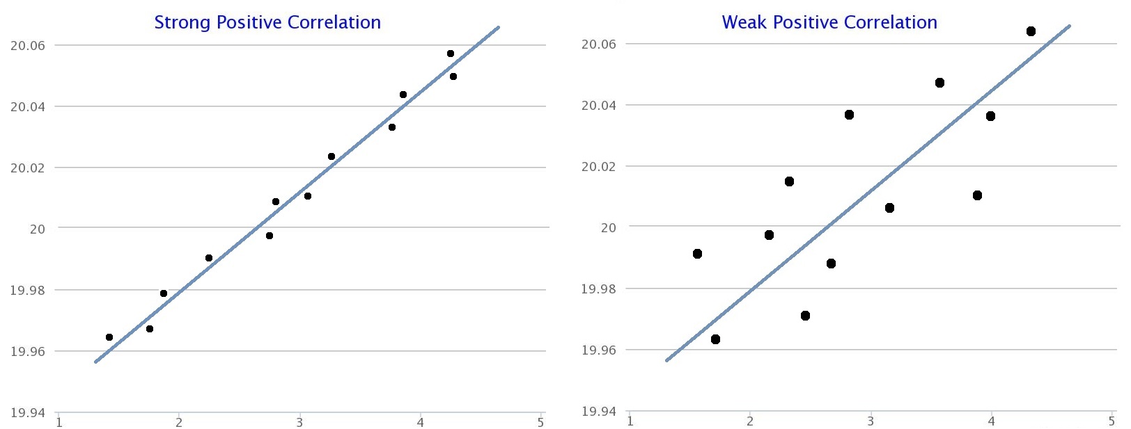
|center|600px|Strong Positive Correlation and Weak Positive Correlation
The closer the data points are to the line of best fit on a scatter graph, the stronger the correlation. It can be measured numerically by a correlation coefficient. There are several coefficients that we use, here are two examples:
- Pearson's Product Moment Correlation Coefficient - measures the strength of the linear correlation between two variables.
- Spearman's Rank Correlation Coefficient - measures the strength of the monotonic correlation between two variables.
Pearson's Product Moment Correlation Coefficient, $r$
Pearson's product moment correlation coefficient (sometimes known as PPMCC or PCC,) is a measure of the linear relationship between two variables that have been measured on interval or ratio scales. It can only be used to measure the relationship between two variables which are both normally distributed. It is usually denoted by $r$ and it can only take values between $-1$ and $1$.
Below is a table of how to interpret the $r$ value.
$r$ value |
Interpretation |
|---|---|
$r = 1$ |
Perfect positive linear correlation |
$1 > r ≥ 0.8$ |
Strong positive linear correlation |
$0.8 > r ≥ 0.4$ |
Moderate positive linear correlation |
$0.4 > r > 0$ |
Weak positive linear correlation |
$r = 0$ |
No correlation |
$0 > r ≥ -0.4$ |
Weak negative linear correlation |
$-0.4 > r ≥ -0.8$ |
Moderate negative linear correlation |
$-0.8 > r > -1$ |
Strong negative linear correlation |
$r = -1$ |
Perfect negative linear correlation |

|1100 px
How To Calculate Pearson's Correlation Coefficient
1. Plot the scatter diagram for your data; you have to do this first to detect any outliers. If you do not exclude these outliers in your calculation, the correlation coefficient will be misleading. By being able to see the distribution of your data you will get a good idea of the strength of correlation of your data before you calculate the correlation coefficient.
2. Next you need to check that your data meets all the calculation criteria. The variables need to be:
- Measured on an interval/ratio scale (like height in inches and weight in kilograms) - this can be checked by looking at the units of the variable you are measuring.
- Normally distributed - you can check this by looking at a boxplot of your data. If the boxplot is approximately symmetric, it is likely that the data will be normally distributed.
- Linearly correlated - look at a significance test of the null and alternative hypothesis.
3. Finally you can calculate the correlation coefficient using the following formula: \[\displaystyle r = \frac{\sum(x_i-\bar x)(y_i-\bar y)}{\sqrt{\sum(x_i-\bar x)^2\sum(y_i-\bar y)^2}},\] where:
- $x_i$ and $y_i$ are your data points,
- $\bar x$ is the mean of the $x$-values and $\bar y$ is the mean of the $y$-values,
- $\sum$ is the summation sign, see sigma notation for more information.
The formula can also be seen in other forms such as: \[\displaystyle r = \frac{Sxy}{\sqrt{Sxx \times Syy}},\] where:
- $Sxy = \sum(x_i-\bar x)(y_i-\bar y) = \sum(xy)-\frac{\sum{x} \sum{y}}{n}$,
- $Sxx = \sum(x_i-\bar x)^2 = \sum(x_i-\bar x)(x_i-\bar x) = \sum(x^2)-\frac{(\sum{x})^2}{n}$,
- $Syy = \sum(y_i-\bar y)^2 = \sum(y_i-\bar y)(y_i-\bar y) =\sum(y^2)-\frac{(\sum{y})^2}{n}$.
Worked Example
Worked Example
Find Pearson's correlation coefficient of the following data:
|
Test score (out of 10) |
Hours playing video games per week |
|---|---|
|
$8$ |
$2$ |
|
$3$ |
$2$ |
|
$5$ |
$1.5$ |
|
$7$ |
$1$ |
|
$1$ |
$2.5$ |
|
$2$ |
$3$ |
|
$6$ |
$1.5$ |
|
$7$ |
$2$ |
|
$4$ |
$2$ |
|
$9$ |
$1.5$ |
Solution

|250px
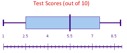
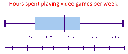
1. First draw the scatter graph. As you can see from the scatter plot, the variables are negatively correlated. You can also see that there are
|250px
|250px
2. Next we need to check that our data meets the calculation criteria:
- Measured on an interval/ratio scale - the variables are measured on an interval scale as they are measured in integers and hours.
- Normally distributed - the boxplots indicate that the two variables are both normally distributed.
- Linearly correlated - the scatter diagram shows that these are linearly correlated, but this could also be checked using a significance test.
3. Finally we can calculate the correlation coefficient using the following formula:
\[r = \frac{\sum(x_i-\bar x)(y_i-\bar y)}{\sqrt{\sum(x_i-\bar x)^2\sum(y_i-\bar y)^2} ~}.\]
Label your variables $x$ and $y$ as it is easier to work with letters compared to names of variables. In this example denote 'test score (out of 10)' by $x$ and 'hours playing video games per week' by $y$.
Start by finding the mean of $x$ and $y$;
\begin{align} \bar{x}&=\frac{\sum{x} }{n}=\frac{8+3+5+7+1+2+6+7+4+9}{10}=\frac{52}{10}=5.2\\ \bar{y}&=\frac{\sum{x} }{n}=\frac{2+2+1.5+1+2.5+3+1.5+2+2+1.5}{10}=\frac{19}{10}=1.9 \end{align}
The easiest way to calculate this is to make a table with all the information you need to put into the formula.
|
$x_i$ |
$y_i$ |
$x_i-\bar x$ |
$y_i-\bar y$ |
$(x_i-\bar x)(y_i-\bar y)$ |
$(x_i-\bar x)^2$ |
$(y_i-\bar y)^2$ |
|---|---|---|---|---|---|---|
|
$8$ |
$2$ |
$8-5.2=2.8$ |
$2-1.9=0.1$ |
$2.8\times 0.1=0.28$ |
$2.8^2=7.84$ |
$0.1^2=0.01$ |
|
$3$ |
$2$ |
$3-5.2=-2.2$ |
$2-1.9=0.1$ |
$-2.2\times 0.1=-0.22$ |
$-2.2^2=4.84$ |
$0.1^2=0.01$ |
|
$5$ |
$1.5$ |
$5-5.2=-0.2$ |
$1.5-1.9=-0.4$ |
$-0.2\times-0.4=0.08$ |
$-0.2^2=0.04$ |
$-0.4^2=0.16$ |
|
$7$ |
$1$ |
$7-5.2=1.8$ |
$1-1.9=-0.9$ |
$1.8\times-0.9=-1.62$ |
$1.8^2=3.24$ |
$-0.9^2=0.81$ |
|
$1$ |
$2.5$ |
$1-5.2=-4.2$ |
$2.5-1.9=0.6$ |
$-4.2\times 0.6=-2.52$ |
$-4.2^2=17.64$ |
$0.6^2=0.36$ |
|
$2$ |
$3$ |
$2-5.2=-3.2$ |
$3-1.9=1.1$ |
$-3.2\times 1.1=-3.52$ |
$-3.2^2=10.24$ |
$1.1^2=1.21$ |
|
$6$ |
$1.5$ |
$6-5.2=0.8$ |
$1.5-1.9=-0.4$ |
$0.8\times-0.4=-0.32$ |
$0.8^2=0.64$ |
$-0.4^2=0.16$ |
|
$7$ |
$2$ |
$7-5.2=1.8$ |
$2-1.9=0.1$ |
$1.8\times 0.8=0.18$ |
$1.8^2=3.24$ |
$0.1^2=0.01$ |
|
$4$ |
$2$ |
$4-5.2=-1.2$ |
$2-1.9=0.1$ |
$-1.2\times 0.1=-0.12$ |
$-1.2^2=1.44$ |
$0.1^2=0.01$ |
|
$9$ |
$1.5$ |
$9-5.2=3.8$ |
$1.5-1.9=-0.4$ |
$3.8\times-0.4=-1.52$ |
$3.8^2=14.44$ |
$-0.4^2=0.16$ |
|
$\sum{x}=52$ |
$\sum{y} = 19$ |
$\sum{(x_i-\bar x)(y_i-\bar y)}=-9.3$ |
$\sum{(x_i-\bar x)^2}=63.6$ |
$\sum{(y_i-\bar y)^2}=2.9$ |
Now we can put all our numbers in our formula to find $r$;
\begin{align} \displaystyle r &= \frac{\sum(x_i-\bar x)(y_i-\bar y)}{\sqrt{\sum(x_i-\bar x)^2\sum(y_i-\bar y)^2}~}\\ &=\frac{-9.3}{\sqrt{63.6\times2.9}~}\\ & =-0.68478681816...\\ &=-0.685\ \text{(3.d.p.)} \end{align}
We can deduce that there is moderate negative linear correlation between test scores (out of 10) and hours playing video games per week.
Note: This does not necessarily mean that the more hours playing video games will reduce your test scores, this simply shows there exists a correlation between them.
Video Example
Alissa Grant-Walker presents a video on finding Pearson's product moment correlation coefficient.
Spearman's Rank Correlation Coefficient, ρ
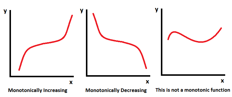
Spearman's coefficient (usually denoted by $ρ$ or $r_s$) is used to measure the monotonic correlation between two variables. A monotonic function is a function of one variable which is either entirely increasing or decreasing.
|250px
Spearman's correlation coefficient technique is applied when your data does not meet the requirements for Pearson's coefficient, for example when the data is skewed or non-linear. Spearman's correlation coefficient can only be applied if the data is on an interval, ratio or ordinal scale (for example if it is ranked 1st, 2nd, 3rd). It can take values between $-1$ and $1$.
Below is a table of how to interpret $\rho$.
ρ value |
Interpretation |
|---|---|
$ρ = 1$ |
Perfect positive monotonic correlation |
$1 > ρ ≥ 0.8$ |
Strong positive monotonic correlation |
$0.8 > ρ ≥ 0.4$ |
Moderate positive monotonic correlation |
$0.4 > ρ > 0$ |
Weak positive monotonic correlation |
$ρ = 0$ |
No correlation |
$0 > ρ ≥ -0.4$ |
Weak negative monotonic correlation |
$-0.4 > ρ ≥ -0.8$ |
Moderate negative monotonic correlation |
$-0.8 > ρ > -1$ |
Strong negative monotonic correlation |
$ρ = -1$ |
Perfect negative monotonic correlation |

|1100px
How To Calculate Spearman's Correlation Coefficient
1. Check that your data is on an interval, ratio or ordinal scale. Draw a scatter graph to check whether your data is monotonic.
2. Rank the data - firstly write all the data in ascending order, then assign the rank 1 to the lowest value and 2 to the second lowest. Continue doing this until all your data is ranked, if you have values which are the same you average the ranks. For example, if you have the values $3,6,8,6,2,4,9$, you would write the numbers in ascending order: $2,3,4,6,6,8,9$. Their ranks would be $1,2,3,4.5,4.5,6,7$ respectively.
3. Calculate the difference between the rank of $x$ and the rank of $y$.
4. Calculate $\rho$ using the formula: \[ρ=1-\frac{6\sum{d^2}}{n(n^2-1)}\]
where:
- $d$ is the difference between the values of rank $x$ and rank $y$,
- $n$ is the number of data pairs in the data set (the number of $x$ or $y$ values),
- $\sum$ is the summation sign, see sigma notation for more information.
Worked Example 2
Worked Example
Find Spearmans's rank correlation coefficient for the following data:
|
Data $x$ |
Data $y$ |
|---|---|
|
$7$ |
$50$ |
|
$3$ |
$19$ |
|
$20$ |
$80$ |
|
$9$ |
$55$ |
|
$11$ |
$66$ |
|
$14$ |
$72$ |
|
$1$ |
$4$ |
|
$4$ |
$36$ |
|
$12$ |
$70$ |
|
$3$ |
$35$ |
Solution
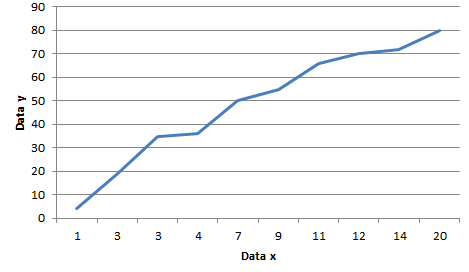
|250px
1. The data is on an interval scale. This is the joined up scatter graph of the data. As the line joining the data is always increasing, the data is monotonically increasing and this means that Spearman's rank correlation coefficient can be used.
2. Rank data $x$ and $y$ and put the results in a table. Start by putting data $x$ and data $y$ in ascending order.
Data $x$:
\[7,3,20,9,11,14,1,4,12,3.\]
Data $x$ in ascending order: \[1,3,3,4,7,9,11,12,14,20,\]
Rank $x$: \[1,2.5,2.5,4,5,6,7,8,9,10,\]
Data $y$: \[50,19,80,55,66,72,4,36,70,35,\]
Data $y$ in ascending order: \[4,19,35,36,50,55,66,70,72,80,\]
Rank $y$: \[1,2,3,4,5,6,7,8,9,10.\]
|
Data $x$ |
Data $y$ |
Rank $x$ |
Rank $y$ |
|---|---|---|---|
|
$7$ |
$50$ |
$5$ |
$5$ |
|
$3$ |
$19$ |
$2.5$ |
$2$ |
|
$20$ |
$80$ |
$10$ |
$10$ |
|
$9$ |
$55$ |
$6$ |
$6$ |
|
$11$ |
$66$ |
$7$ |
$7$ |
|
$14$ |
$72$ |
$9$ |
$9$ |
|
$1$ |
$4$ |
$1$ |
$1$ |
|
$4$ |
$36$ |
$4$ |
$4$ |
|
$12$ |
$70$ |
$8$ |
$8$ |
|
$3$ |
$35$ |
$2.5$ |
$3$ |
3. Find the difference between $x$ and $y$ and label this $d$. Calculate $d^2$ and $\sum{d^2}$.
|
Data $x$ |
Data $y$ |
Rank $x$ |
Rank $y$ |
$d$ |
$d^2$ |
|---|---|---|---|---|---|
|
$7$ |
$50$ |
$5$ |
$5$ |
$0$ |
$0$ |
|
$3$ |
$19$ |
$2.5$ |
$2$ |
$0.5$ |
$0.25$ |
|
$20$ |
$80$ |
$10$ |
$10$ |
$0$ |
$0$ |
|
$9$ |
$55$ |
$6$ |
$6$ |
$0$ |
$0$ |
|
$11$ |
$66$ |
$7$ |
$7$ |
$0$ |
$0$ |
|
$14$ |
$72$ |
$9$ |
$9$ |
$0$ |
$0$ |
|
$1$ |
$4$ |
$1$ |
$1$ |
$0$ |
$0$ |
|
$4$ |
$36$ |
$4$ |
$4$ |
$0$ |
$0$ |
|
$12$ |
$70$ |
$8$ |
$8$ |
$0$ |
$0$ |
|
$3$ |
$35$ |
$2.5$ |
$3$ |
$0.5$ |
$0.25$ |
|
$\sum{d^2}=0.5$ |
4. Apply the formula: \[ρ=1-\frac{6\sum{d^2} }{n(n^2-1)}=1-\frac{6\times{0.5} }{10(10^2-1)}=1-\frac{3}{990}=1-0.00303=0.997\ \text{(3.d.p.)}\]
We can deduce by this that there is a very strong positive monotonic correlation between data $x$ and data $y$.
Video Example
This is a worked example calculating Spearman's correlation coefficient produced by Alissa Grant-Walker.
Workbook
This workbook produced by HELM is a good revision aid, containing key points for revision and many worked examples.
Test Yourself
Test yourself: Numbas test on measures of correlation
External Resources
- Correlation at
- Presentation on Pearson's Correlation at
- Spearman's Correlation at
- Presentation on Spearman's Correlation at