Solving Simultaneous Linear Equations (Economics)
Solving Simultaneous Linear Equations
Two or more linear equations that all contain the same unknown variables are called a system of simultaneous linear equations. Solving such a system means finding values for the unknown variables which satisfy all the equations at the same time.
See below for examples of where we use simultaneous equations in economics.
There are two common methods for solving simultaneous linear equations: substitution and elimination. In some questions, one method is the more obvious choice, often because it makes the process of solving the equations simpler; in others, the choice of method is up to personal preference. In either case, both methods would eventually lead to the same solution.
Note: To be able to solve any system of linear equations we must have at least as many equations as we have variables.
Here we shall focus on systems with two equations and two variables.
How Many Solutions?
A system of simultaneous linear equations can have either: one unique solution, infinitely many solutions or no solutions.
We know that the graph of a linear equation is a straight line so a system of two linear equations has two straight lines. If these lines:
1) Intersect there is one unique solution to the system of equations. This makes sense as there can only pair of values (one for each variable) which satisfy both equations at the same time. This pair of value will correspond to the point of intersection.
2) Are the same line there are said to be infinitely many solutions to the system of equations: all pairs of values for the variables on one line satisfy the equation of the other line as they are the same line.
3) Are parallel there are no solutions: there are no pairs of values of $x$ and $y$ which lie on both lines (as the lines can never cross!) and so there can be no pairs of values for the variables which satisfy both equations.
One way to determine whether a system of two linear equations can be solved and how many solutions it has is to arrange both equations into the form: \[y=ax+b\] where $a$ is the slope of the line and $b$ is the $y$-axis intercept. It should now be clear whether the two equations correspond to either:
1) Different and non-parallel lines (different slopes), so there is one unique solution.
2) The same line (same slope and intercept), and so there are infinitely many solutions.
3) Parallel lines (they have the same slope but a different intercept), and so there are no solutions.
The Substitution Method
The substitution method involves substituting one equation into another in order to eliminate one of the variables. We can then solve for the other variable. The next step is to substitute the value of this variable into one of the equations to determine the value of the other variable. Note that this may involve rearranging one of the equations so that is it in a form which can easily be substituted into the other equation.
Worked Example
Solve this pair of linear simultaneous equations
\begin{align} y\,-\,2x &= 1\\ 2y-3x &=5 \end{align}
Solution
It's a good idea to label the equations so they're easier to refer to. \begin{align} y\,-\,2x &= 1 & \textbf{(1)} \\ 2y-3x &=5 & \textbf{(2)} \end{align}
The first step is then to rearrange equations $(1)$ and $(2)$ into the form $y=ax+b$. This gives: \begin{align} y&=2x+1 & \textbf{(3)} \\ y&=\frac{3}{2}x+\frac{5}{2} & \textbf{(4)} \end{align}
where equation $\textbf{(3)}$ corresponds to equation $\textbf{(1)}$ and equation $\textbf{(4)}$ corresponds to equation $\textbf{(2)}$. We can now see that the two equations correspond to different and non-parallel lines (as they have different slopes) and so there is one unique solution to this system of equations. We will now solve this system using the substitution method.
Substituting equation $\textbf{(3)}$ into equation $\textbf{(2)}$ gives:
\[2(1+2x)-3x=5\] Note: We can substitute equation $\textbf{(3)}$ into equation $\textbf{(2)}$ because equation $\textbf{(3)}$ is just a rearranged version of equation $\textbf{(1)}$. We could also have substituted equation $\textbf{(4)}$ into equation $\textbf{(1)}$. However we could not have substituted equation $\textbf{(3)}$ into equation $\textbf{(1)}$ (or $\textbf{(4)}$ into $\textbf{(2)}$) because they are the same equation.
Now we have an equation in only one variable, which can be rearranged and solved to find $x$.
\begin{align} 2(1+2x)-3x&=5 \\ 2+4x-3x&=5\\ 2+x&=5\\ x&=3 \end{align}
Now we have a value for $x$, this can be substituted into either of the original equations to find $y$. It's easiest to use the rearranged for of equation $\textbf{(1)}$ (equation $\textbf{(3)}$):
\[y= 2\times 3+1=7.\]
The solution $x=3$ and $y=7$ satisfies both equations. It's a good idea to check your solution by substituting these values of $x$ and $y$ into the original equations.
\begin{align} y - 2x &= 1 & \textbf{(1)}\\ 7 - 2 \times 3 &= 7 - 6 = 1. \\ \\ 2y - 3x &= 5 & \textbf{(2)}\\ 2 \times 7 - 3 \times 3 &= 14 - 9 = 5. \end{align}

|center
This graph shows the lines $y-2x=1$ and $2y-3x=5$. The solution to these simultaneous equations is the point at which the two lines intersect. We can see that this is the point $(3,7)$, which agrees with our solution.
Worked Example
Solve this system of two simultaneous linear equations.
\begin{align} 5y-2x=45\\ 6x=15y-135 \end{align}
Solution
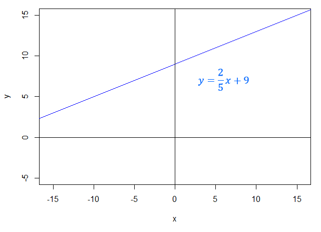
Rearranging the two equations into the form $y=ax+b$ gives: \begin{align} y=&\dfrac{2x}{5}+9\\ y&=\dfrac{2x}{5}+9 \end{align}
The lines are the same, so there are infinitely many solutions.
Video Example
Prof. Robin Johnson uses the substitution method to solve the simultaneous equations $3x-2y=7$ and $y+4x=5$.
Elimination
Definition
When given two simultaneous linear equations with two unknowns, we can also apply the elimination method. The elimination method involves choosing a variable to eliminate.
Start by multiplying both equations by appropriate constants so that in each equation the chosen variable has the same coefficient (disregarding its sign: whether it is positive or negative).
Then, depending on the sign of the coefficient of this same variable, either add or subtract one equation from the other so that the terms involving the variable to be eliminated cancel out.
The remaining equation is in one variable, and can be solved in the usual way; the value of that variable is then substituted into one of the original equations to find the value of the eliminated variable.
Worked Examples
Worked Example
Solve the simultaneous linear equations
\begin{align} 2x+y &= 7 \\ 3x-y &= 8 \end{align}
Solution
Rearranging the two equations into the form $y=ax+b$ gives: \begin{align} y=&-2x+7\\ y&=3x-8 \end{align}
The lines have different slopes, so there is one unique solution. We will now find it using the elimination method.
Let's first label the equations: \begin{align} 2x+y &= 7 & \textbf{(1)} \\ 3x-y &= 8 & \textbf{(2)} \end{align}
Notice here that the coefficient of $y$ is the same up to sign in both of the equations. As one is positive and one is negative, if we add the two equations together, the $y$'s will cancel.
\begin{align} &2x+y=7\\ &3x-y=8\\ &\overline{5x \quad\;\;\, = 15} \end{align}
So $x=3$.
Now substitute this value for $x$ back into equation $\textbf{(1)}$.
\begin{align} 2x + y &= 7 \\ 2\times 3+y&=7\\ 6+y &=7\\ y&=1 \end{align}
The values $x=3$, $y=1$ satisfy both of the equations we were given.

|center
This graph shows the lines $2x+y=7$ and $3x-y=8$. The solution to these simultaneous equations is the point at which the two lines intersect. We can see that this is the point (3,1) which agrees with our solution.
Worked Example
Solve this system of two simultaneous linear equations.
\begin{align} 2x + 3y &= 4 \\ x - 2y &= -5 \end{align}
Solution
Rearranging the two equations into the form $y=ax+b$ gives: \begin{align} y=&-\dfrac{2x}{3}+\frac{4}{3}\\ y&=\dfrac{x}{2}+\frac{5}{2} \end{align}
The lines have different slopes, so there is one unique solution. We will now find it using the elimination method. First label the equations 1 and 2, respectively.
\begin{align} 2x + 3y &= 4 & \textbf{(1)} \\ x - 2y &= -5 & \textbf{(2)} \end{align}
We want to make the coefficients of $x$ the same in both equations. To do this, multiply equation (2) by $2$.
\[2x-4y=-10\]
As the coefficients of $x$ in both equations are positive, we subtract equation 2 from equation 1.
\begin{align} &2x+3y=4\\ &2x-4y=-10\\ &\overline{\qquad \; 7y =14} \end{align}
So $y=2$.
Substituting this value for $y$ back into one of the original equations will give $x$.
\begin{align} x - 2y &= -5 & \textbf{(2)} \\ x-2\times 2&=-5\\ x-4&=-5\\ x&=-1 \end{align}
The values $x=-1$ and $y=2$ satisfy both of the equations we were given.

|center
This graph shows the lines $2x+3y=4$ and $x-2y=-5$. The solution to these simultaneous equations is the point at which the two lines intersect.
Worked Example
Solve this system of two simultaneous linear equations.
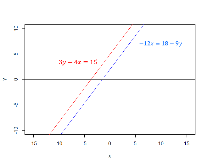
\begin{align} 3y-4x=15\\ -12x=18-9y \end{align}
Solution
Rearranging the two equations into the form $y=ax+b$ gives: \begin{align} y=&-\dfrac{4x}{3}+5\\ y&=\dfrac{4x}{3}+2 \end{align}
The lines have the same slope but different $y$-intercepts (they are parallel), so there are no solutions as they never intersect.
Applications of Simultaneous Linear Equations in Economics
Demand and Supply
The above methods for solving pairs of simultaneous linear equations can used to find the market equilibrium when we have linear market supply and market demand functions. For example, suppose that in a small economy the market demand and supply functions for bananas are: \begin{align} &q^S=5p-25\\ &q^D=-2p+24 \end{align} where $q^D$ is the quantity of bananas demanded (in kilos), $q^S$ is the quantity of bananas supplied (in kilos) and $p$ is the price per kilo of bananas (in $£$).
This market is in equilibrium when the quantity demanded is equal to the quantity supplied: \[q^D=q^S\] As here we are only interested in this market when it is in equilibrium, in order to solve the system of equations we can set both $q^D$ and $q^S$ equal to $q$. The demand and supply functions then become: \begin{align} &q=5p-25 & \textbf{(1)}\\ &q=-2p+24 & \textbf{(2)} \end{align} To find the equilibrium, we can use either of the above methods to find the values of the variables $q$ and $p$ which satisfy both of these functions. Here we will use the substitution method.
Substituting equation $\textbf{(1)}$ into equation $\textbf{(2)}$ gives: \begin{align} 5p-25&=-2p+24\\ \Rightarrow 7p&=49\\ \Rightarrow p&=7 \end{align}
Substituting this value of $p$ into equation $\textbf{(1)}$ gives: \begin{align} q&=5\times 7-25\\ \Rightarrow q&=10 \end{align}
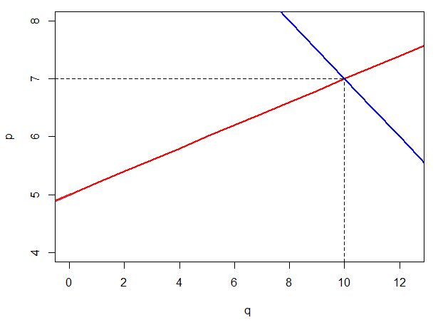
So the solution to this system of equations is $q=10$ and $p=7$. This solution is shown graphically below, where we have plotted the inverse demand function (in blue) and the inverse supply function (in red) on the same graph. We can see that the equilibrium corresponds to the intersection of these two functions. That is, the point where $q=10$ and $p=7$.
Inverse Demand and Supply Equations
Rearranging supply and demand functions to make $p$ the subject gives us what is know as the inverse supply and demand functions. In economics we typically put price on the vertical axis, so in order to plot supply and demand functions, we must first find their inverses.
Consider again the market for bananas from above. Suppose that instead we were given the inverse demand and supply functions: \begin{align} &p^S=\dfrac{q^S}{5}+5\\ &p^D=-\dfrac{q^D}{2}+12 \end{align} and asked to find the market equilibrium.
We now appear to have two equations and four unknowns. However, since there can only be one equilibrium price and one equilibrium quantity, in equilibrium we must have: \[p^D=p^S\text{ and }q^D=q^S\] As we are only interested in this market when it is in equilibrium, to solve the system of equations we can therefore set both $p^D=p^S\text{ and }q^D=q^S$. The two functions then become: \begin{align} &p=\dfrac{q}{5}+5\\ &p=-\dfrac{q}{2}+12 \end{align} We now have two equations and two unknowns and so can solve this system of equations. Try this for yourself (hint: you should get the same values for $p$ and $q$ as above).
Comparative Statics
An example of comparative statics is the effect of a tax. Here we will consider $2$ types of tax: per-unit tax and ad valorem tax.
Per-Unit Tax
A per-unit or specific tax is a fixed amount which is charged for each unit of a good or service sold. For instance, suppose that in the market for bananas considered above, the government imposes a per-unit tax of $£1$ per kilo on sellers.
Taking the inverse of the supply function from above we have: \[p^S=\dfrac{q^S}{5}+5\] With the tax, sellers must now be paid $T=£0.70$ more for each kilo of bananas that they produce (to cover their additional costs from the tax) so the tax-modified inverse supply function is: \begin{align} p^S&=\dfrac{q^S}{5}+5+0.7\\ &=\dfrac{q^S}{5}+5.7 \end{align} The tax has no effect on the demand function as the consumers do not pay the tax, so we have: \[p^D=-\dfrac{q^S}{2}+12\] As usual, in equilibrium we have $p^D=p^S\text{ and }q^D=q^S$, so to find the market equilibrium we can write the demand and (tax-modified) supply functions as: \begin{align} &p=\dfrac{q}{5}+5.7 & \textbf{(1)}\\ &p=-\dfrac{q}{2}+12 & \textbf{(2)}\\ \end{align} Since both equations have different slopes, the system is solvable. We will now solve this system of equations using the substitution method. Rearranging equation $\textbf{(1)}$ to make $q$ the subject gives: \begin{align} \dfrac{q}{5}&=p-5.7\\ \Rightarrow q&=5p-28.5& \textbf{(3)}\\ \end{align} We can now substitute equation $\textbf{(3)}$ into equation $\textbf{(2)}$ as follows: \begin{align} &p=-\dfrac{5p-28.5}{2}+12\\ \Rightarrow &2p=-5p+28.5+24\\ \Rightarrow &7p=52.5\\ \Rightarrow &p=7.5\\ \end{align}
Substituting this value of $p$ into equation $\textbf{(3)}$ gives: \begin{align} q&=5\times 7.5-28.5\\ &=9 \end{align}
So with the tax levied on producers, the equilibrium quantity has dropped from $10$ kilos to $9$ kilos and the equilibrium price has risen from $£7$ to $£7.05$ per kilo.
In the above graph we can see that the tax has the effect of shifting the supply curve leftwards. Consequently, the equilibrium point (the intersection of the tax-modified supply function and the demand function) has also shifted leftwards.
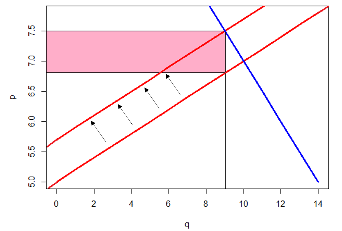
To work out the revenue generated from this tax, we multiply the amount of tax per unit by the quantity produced in equilibrium: \[\text{tax}=£(0.70\times 9)=£6.30\] This is equal to the area of the shaded pink rectangle shown in the above graph.
Ad Valorem Tax
An ad valorem tax is levied as a percentage of the quantity of the good or service being taxed.
For example, suppose that in the market for bananas (see above) the government decides to impose an ad valorem tax of $5\%$ on sellers . The original inverse supply function was: \[p^S=\dfrac{q^S}{5}+5\] so the tax-modified inverse supply function becomes: \begin{align} p^S&=(1+0.05)\left(\dfrac{q^S}{5}+5\right)\\ &=1.05\left(\dfrac{q^S}{5}+5\right)\\ &=0.21q^S+5.25 \end{align} As usual, in equilibrium we have $p^D=p^S\text{ and }q^D=q^S$, so to find the market equilibrium we can write the demand and (tax-modified) supply functions as: \begin{align} &p=0.21q+5.25 & \textbf{(1)}\\ &p=-\dfrac{q}{2}+12 & \textbf{(2)}\\ \end{align} Since both equations have different slopes, the system is solvable. We will now solve this system of equations using the substitution method. Rearranging equation $(2)$ to make $q$ the subject gives: \[q=-2p+24\;\;\; \textbf{(3)}\] Substituting equation $(3)$ into equation $(1)$ gives: \begin{align} p&=0.21(-2p+24)+5.25\\ &=-0.42p+10.29\\ &\Rightarrow 1.42p=10.29\\ &\Rightarrow p=7.246... \end{align}
Substituting this value of $p$ into equation $(3)$ gives: \begin{align} q&=-2\times 7.246...+24\\ &=9.507... \end{align}
So the new equilibrium price and quantity of bananas (to $2$d.p.) are $p=7.25$ and $q=9.51$. In other words, the equilibrium price of bananas (in $£$) is $£7.25$ and the equilibrium quantity is $9.51$ kilos. To calculate the revenue raised from the ad valorem tax we must find the product of the equilibrium quantity and the amount of the tax:
$0.05\times 9.507...=0.48$ (to $2$d.p.)
So the tax revenue is $£0.48$.
Input-Output Analysis
Input-output analysis is used to show how industries in the same economy are interrelated. In particular, it shows how the output of one industry is often used as an input for another industry and that the output of an industry can be used as an input for that same industry. For simplicity we will assume here that an economy can have only $2$ industries.
For example, consider an economy which produces coal $\left(X\right)$ and steel $\left(Y\right)$. Coal is needed to produce steel and steel is used to make the tools needed to produce coal: the industries are interrelated.
Suppose that producing a single unit ($1$kg) of coal requires $0.18$kg of coal and $0.03$kg of steel, while producing a single unit ($1$kg) of steel requires $0.21$kg of coal and $0.04$kg of steel. We can express this information in the form of a table:
$X$ |
$Y$ |
|
|---|---|---|
$X$ |
$0.18$ |
$0.03$ |
$Y$ |
$0.21$ |
$0.04$ |
Another way to express this information is in the form of equations: \begin{align} x^*&=x-0.18x-0.03y\\ y^*&=y-0.21x-0.04y\\ \end{align} where $x$ and $y$ are the total amounts (in kg) or gross output of coal and steel produced and $x^*$ and $y^*$ are the net amounts (in kg) of steel and coal produced.
Now, suppose that to satisfy the consumption needs of this economy, $36.06$kg of steel and $26.53$kg of coal must be produced. This is the net output of steel and coal respectively and so we can rewrite (and label) the above equations as: \begin{align} 26.53&=0.82x-0.03y & \textbf{(1)} \\ 36.06&=0.96y-0.21x& \textbf{(2)} \\ \end{align} We now have a system of simultaneous linear equations which we can solve using either of the above methods. As usual, the first step is to rewrite the equations in the form $y=mx+c$. This gives: \begin{align} y&=\dfrac{82x}{3}-\dfrac{26.53}{0.03} & \textbf{(3)}\\ y&=\dfrac{7x}{32}+\frac{36.06}{0.96} & \textbf{(4)}\\ \end{align}
Since the lines have different slopes, there is a unique solution to this system of equations. Here we will use the substitution method. Substituting equation $\textbf{(4)}$ into equation $\textbf{(1)}$ gives: \begin{align} 26.53&=0.82x-0.03\left(\dfrac{7x}{32}+\frac{36.06}{0.96}\right)\\ \Rightarrow x&=34 \end{align} We can now substitute this value of $x$ can into either equation $\textbf{(3)}$ or $\textbf{(4)}$ to find the value of $y$. Substituting $x=34$ into equation $\textbf{(3)}$ gives: \begin{align} y&=\dfrac{82\times 34}{3}-\dfrac{26.53}{0.03}\\ &=45 \end{align}
The gross amount of coal and steel which needs to be produced in order to satisfy the consumption needs of this economy are $34$kg of coal and $45$kg of steel.
Macroeconomic Equilibrium
Here we will look at how methods for solving systems of simultaneous equations can be used to determine the equilibrium level of income for the whole economy. To do this, we must first consider the key relationships in our model of the economy.
If we make the simplifying assumption that households earn their income based solely upon how much output they produce, then aggregate household income $Y$ must equal output $Q$. We can write this as an identity \[Y\equiv Q\] If we also assume that all output is purchased by someone we have that output $Q$ is equal to demand or aggregate expenditure $E$, so: \[Q\equiv E\] Combining the above equations gives: \[Y\equiv E\;\;\;\textbf{(1)}\] Now, since aggregate expenditure is made up of consumption expenditure by households $C$ and investment expenditure by firms $I$, we have another identity: \[E\equiv C+I\;\;\;\textbf{(2)}\]
The consumption function says that planned household consumption $\hat{C}$ is a function of household income. If we assume that this relationship is linear, then we can write: \[\hat{C}=aY+b\;\;\;\textbf{(3)}\] where $a$ and $b$ are both positive constants and $a\lt 1$.
Note: $a$ is the slope of the consumption function and is also called the marginal propensity to consume (MPC). The value of $a$ tells us the proportion of an aggregate rise in income that will be spent on the consumption of goods and services. $b$ is the intercept term.
In equilibrium planned household consumption must be equal to actual household consumption: \[C=\hat{C}\;\;\;\textbf{(4)}\]
Now, if we assume that investment expenditure is equal to some fixed value $\hat{I}$, we can write: \[I=\hat{I}\;\;\;\textbf{(5)}\] and so equation $\textbf{(2)}$ can be written as: \[E\equiv C+\hat{I}\;\;\;\textbf{(2)}\]
Equations $\textbf{(1)}$ to $\textbf{(5)}$ make up our macroeconomic model. However, we can simplify this model by combining equations to reducing the number of them. Combining equation $\textbf{(1)}$ with equation $\textbf{(2)}$ gives: \[Y\equiv C+\hat{I}\;\;\;\textbf{(1.1})\] Next we can combine equations $\textbf{(3)}$ and $\textbf{(4)}$ to get: \[C=aY+b\;\;\;\textbf{(1.2})\] We now have $2$ equations (equation $\textbf{(1.1)}$ and equation $\textbf{(1.2)}$) and $2$ unknowns ($C$ and $Y$) so we can use the above methods to solve this system of equations. Here we will use the substitution method. Substituting equation $\textbf{(1.1})$ into equation $\textbf{(1.2})$ gives: \begin{align} Y&=(aY+b)+\hat{I}\\ \Rightarrow (1&-a)Y=b+\hat{I}\\ \Rightarrow Y&=\dfrac{b+\hat{I}}{1-a} \end{align} This tells us that the equilibrium level of income is equal to the sum of the intercept term $b$ and investment, divided by $1$ minus the MPC.
Worked Example
Given the following macroeconomic model: \begin{align} Y&\equiv E\\ E&\equiv C+I\\ \hat{C}&=0.25Y+50\\ I&=250\\ C&=\hat{C} \end{align}
a) Find the equilibrium levels of income and consumption, and illustrate diagrammatically.
b) If investment rises to $550$ find the new equilibrium levels of income and consumption.
Solution
a) As for the general model, we can simplify this model of the economy by combining equations to reducing the number of them. Combining the second equation with the first gives: \[Y\equiv C+250\;\;\;\textbf{(1)}\] where $250$ has been substituted for $I$. Combining the third equation with the fifth gives: \[C=0.25Y+50\;\;\;\textbf{(2)}\] We now have $2$ equations and $2$ unknowns so we can solve the system of equations. Substituting equation $\textbf{(2)}$ into equation $\textbf{(1)}$ gives: \begin{align} Y&=(0.25Y+50)+250\\ &=0.25Y+300\\ \Rightarrow 0.75Y&=300\\ \Rightarrow Y&=400 \end{align} and substituting this value of $Y$ into equation $\textbf{(2)}$ gives: \begin{align} C&=0.25\times 400+50\\ &=150 \end{align} so the equilibrium level of income is $Y=400$ and the equilibrium level of consumption is $C=150$.
b) If investment rises to $400$, equation $\textbf{(1)}$ from part a) becomes: \[Y\equiv C+550\;\;\;\textbf{(1.1)}\] and equation $\textbf{(2)}$ remains unchanged as it does not contain an $I$ term: \[C=0.25Y+50\;\;\;\textbf{(2.1)}\] We will now use the substitution method to solve these equations. Substituting equation $\textbf{(2)}$ into equation $\textbf{(1)}$ gives: \begin{align} Y&=(0.25Y+50)+550\\ &=0.25Y+600\\ \Rightarrow 0.75Y&=600\\ \Rightarrow Y&=450 \end{align} and substituting this value of $Y$ into equation $\textbf{(2.1)}$ gives: \begin{align} C&=0.25\times 450+50\\ &=162.50 \end{align} so when investment rises to $550$ the equilibrium level of income rises to $Y=450$ and the equilibrium level of consumption rises to $C=162.50$. This makes sense as investment is part of aggregate demand, so when investment rises output and therefore aggregate income should also rise.
Video Example
Prof. Robin Johnson solves the simultaneous equations $2x-3y=5$ and $7x+2y=1$ using the elimination method.
Workbook
This workbook produced by HELM is a good revision aid, containing key points for revision and many worked examples.
Test Yourself
Test yourself: Numbas test on simultaneous equations