Non-parametric Hypothesis Tests (Psychology)
What is a Non-parametric Test?
Parametric hypothesis tests are based on the assumption that the data of interest has an underlying Normal distribution. The Normal distribution has the form of a symmetric bell-shaped curve, so naturally we need our data to be symmetric for a parametric test to be appropriate. However, sometimes our data is asymmetric so we must use a non-parametric test.
It is a traditional alternative approach because it makes few or no assumptions about the distribution of the data or population. Many non-parametric tests are based on ranks given to the original numerical scores/data. Usually non-parametric tests are regarded as relatively easy to perform but some problems can occur. It can be cumbersome to carry out such tests when working with large amounts of data. In psychological data, there are quite restricted ranges of scores, which can result in the same value appearing several times in a set of data. Tests based on rank can become more complicated with increased tied scores.
Important Note
The examples covered on this page do not necessarily have the best experimental designs. They are also purely hypothetical and any results or data are not from any real studies nor experiments. The purpose of them is to demonstrate how to use the various hypothesis tests covered in this section.
Example: Ranking Data
To rank data we must order a set of scores from smallest to largest. The smallest score is given rank 1, the second smallest score is given 2 and so on. It is purely the sample size that affects the ranks and not the actual numerical values of the scores.
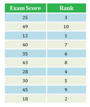
Imagine you have collected a sample of ten students' exam scores (out of fifty) and wish to rank them.
You collect the following scores: $25, 49, 12, 40, 35, 43, 28, 30, 45, 18$.
If we sort them into ascending order, we get: $12, 18, 25, 28, 30, 35, 40, 45, 49$.
These are now in ranked order and we can put them into a table:
|center
Sign Test
The sign test is similar to the paired/related t-test, as it takes the differences between the two related samples of scores. However, you consider the sign of the difference, rather than the size of difference.
The Method
- First, you delete any case where the scores are the same in both groups (so zero differences), they can be ignored in the sign test.
- Subtract the second group's scores away from the first group's. Remember to include the sign of the difference ($+$ or $-$).
- Now count the number of differences which have a positive sign and then count the number of differences with a negative sign.
- Take the smaller number.
- Look up the significance of the smaller number in a significance table. You look at the row containing the sum of the positive and negative signs (the total number of differences ignoring zero differences.) Your value must be in the range specified in the table for it to be statistically significant.
- Report your findings and form your conclusion.
Worked Example
Example 1

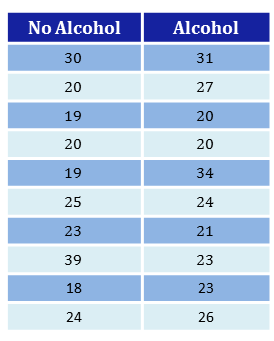
A study has been conducted into the effects of alcohol and reaction time. Ten participants are asked to watch a video and press a button every time a small red circle appears on the screen. The total time between the circles appearing and when the button is pressed is recorded for each participant. If a participant fails to press the button at any time, a time of $5$ seconds is added onto the total time.
A week later the participants are then asked to repeat the task of watching the video and pressing the button when every red circle appears. However, this time they drink an alcoholic drink containing $2$ units of alcohol $15$ minutes beforehand. The total times are recorded again. Below is a table of the resulting times, to the nearest second.
' Perform a hypothesis test to see if alcohol as an effect on reaction times'
|center
Solution
The hypothesis we wish to test is if alcohol has an effect on reaction time. The null hypothesis $H_0$ is that alcohol has no effect on reaction time.
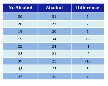
Firstly, remove any rows from the table which have identical scores. In this instance, the fourth participant has the same time under and not under the influence of alcohol. We then calculate the differences by subtracting the first column from the second column.
|center
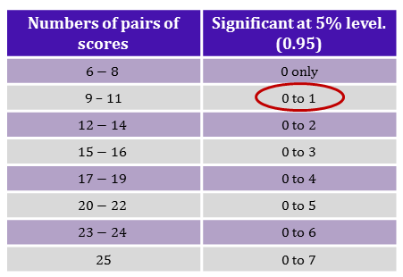
We can count that $2$ differences have a negative sign, whereas $7$ differences have a postive sign. (Remember, we deleted data from one of our ten participants). So we use $2$ as our value to compare with significance tables.
|center
Looking at the $9 - 11$ row, we can see that the smaller number needs to be either $0$ or $1$ to have a significant significant results. Our value is $2$, so our results are not statistically unusual and we accept the null hypothesis. There is not enough evidence to suggest that alcohol has an effect on reaction time. Perhaps a study with more participants should be carried out.
A concise way of reporting our findings could be:
'Reactions times were slightly slower after consuming alcohol $(\bar{X}=24.444)$ (3 d.p.) compared to when alcohol was not consumed $(\bar{X}=24.111)$ (3 d.p.). However, this did not reach statistical significance, so it was not possible to reject the null hypothesis that alcohol has no effect on reaction time in this particular sample $($sign test$, n = 9, p$ ns$)$.'
Note: ns means not significant.
Mann-Whitney U-Test
The Mann-Whitney $U$-test is perhaps the most common non-parametric test for unrelated samples of scores. You would use it when the two groups are independent of each other, for example if you were testing two different groups of people in a conformity study. It can used when the two groups are different sizes and also when they are the same size.
The Method
- First, we state our null and alternative hypotheses.
- Next, we rank all of the scores (from both groups) from the smallest to largest. Equal scores are allocated the average of the ranks they would have if there was tiny differences between them. For example, say there are two scores of $13$. If there was just one score of $13$ it would have the rank $7$ in this particular example. However, since there are two scores of $13$, we instead assign the rank $\dfrac{7+8}{2} = 7.5$ to both scores.
- Next we sum the ranks for each group. You call the sum of the ranks for the larger group $R_1$ and for the smaller sized group, $R_2$. If both groups are equally sized then we can label them whichever way round we like.
- We then input $R_1$ and $R_2$ and also $N_1$ and $N_2$, the respective sizes of each group, into the following formula:
\begin{equation} U = (N_1 \times N_2) + \dfrac{N_1 \times (N_1+1)}{2} - R_1 \end{equation}
- Then we compare the value of $U$ to significance tables. You find the intersection of the column with the value of $N_1$ and the row with the value of $N_2$. In this intersection there will be two ranges of values of $U$ which are significant at the $5\%$ level. If our value is within one of these ranges, then we have a significant result and we reject the null hypothesis. If our value is not in the range then it is not significant and then the independent variable is unrelated to the dependent variable, we accept the $H_0$.
- As a check, we also need to examine the means of the two groups, to see which has the higher scores on the dependent variable.
- We then report our results.
Worked Example
Example 1
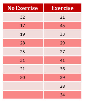
A study into the effect of exercise on memory was carried out. One group (of size $8$) spent an hour sitting in a chair for $15$ minutes (No exercise group), whereas the other group (of size $10$) spent $15$ minutes playing dodgeball (Exercise group). They then were then shown $50$ random objects over a $4$ minute period and then asked to recall as many items as they possibly could in $2$ minutes. The number of objects they could remember was recorded as their scores. The results are in the table below.
Perform a Mann-Whitney $U$-test to see if there is a difference between the two groups.
| center
Solution
Here we have, \begin{align} H_0:& \text{Exercise has no effect on memory}.\\ H_1:& \text{Exercise has an effect on memory}.\\ \end{align} Now we need to assign ranks to each score.
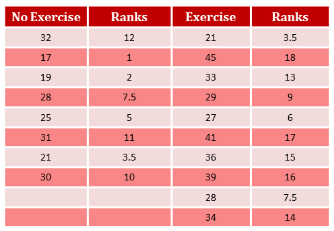
An easy way to do this is write all the scores in ascending order and then write their corresponding ranks next to them and then put these back into a table.
So we have:
\begin{align} 17 - & 1\\ 19 - & 2\\ 21 - & 3.5\\ 21 - & 3.5\\ 25 - & 5\\ 27 - & 6\\ 28 - & 7.5\\ 28 - & 7.5\\ 29 - & 9\\ 30 - & 10\\ 31 - & 11\\ 32 - & 12\\ 33 - & 13\\ 34 - & 14\\ 36 - & 15\\ 39 - & 16\\ 41 - & 17\\ 45 - & 18\\ \end{align}
Note, the two scores of $21$ have a rank of $\frac{(3 + 4)}{2} = 3.5$ and the two scores of $28$ have a rank of $\frac{(7 + 8)}{2} = 7.5$.
We now can arrange these into a table.
|center
Now we can calculate $R_1$ and $R_2$. The 'Exercise' group is larger in size so we use those ranks to calculate $R_1$ and we use the smaller 'No exercise' group's ranks to calculate $R_2$. $N_1 = 10$ and $N_2 = 8$.
\begin{align} R_1 &= 3.5 + 18 + 13 + 9 + 6 + 17 + 15 + 16 + 7.5 + 14\\ &= 119\\ R_2 &= 12 + 1 + 2 + 7.5 + 5 + 11+ 3.5 + 10\\ &= 52.\\ \end{align}
Now we can calculate our $U$-value:
\begin{align} U &= (N_1 \times N_2) + \dfrac{N_1 \times (N_1 +1)}{2} - R_1\\ &= (10 \times 8) + \dfrac{10 \times (10+1)}{2} - 119\\ &= 80 + \dfrac{110}{2} - 119\\ &= 16.\\ \end{align}
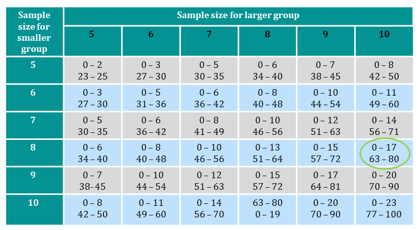
We then compare it to a significance table.
|center
We can see that the $U$ -value of $16$ lies within the range $0 - 17$, thus we have a significant result at the $5\%$ level. This suggests we have evidence that exercise does have an effect on memory. Note: the mean scores for the 'Exercise' and 'No exercise' groups are respectively $25.375$ and $33.3$.
In a report, we would state our findings as follows.
'It was found that the scores of the memory tests were significantly higher $(U=16, n = 18. p<0.05)$ in the exercise group $(\bar{X}=33.3)$ than in the no exercise group$(\bar{X}=25.375)$.'
Wilcoxon Matched Pairs Test
The Wilcoxon matched pairs test, also known as the Wilcoxon signed ranks test, is similar to the sign test. The only alteration is that we rank the differences ignoring their signs (but we do keep a note of them). As the name implies, we use the Wilcoxon matched pairs test on related data, so each sample or group will be equal in size.
The Method
- Calculate the difference scores between your two samples of data. We then remove difference scores of zero.
- Rank them. If scores are tied then you use the same method as in the Mann-Whitney tests. You assign the difference scores the average rank if it was possible to separate the tied difference scores.
- The ranks of the differences can now have the sign of the difference reattached (we will use superscripts - see example below).
- The sum of the positive ranks are calculated.
- The sum of the negative ranks are calculated.
- You then choose the smaller sum of ranks and we call this our $T$-value, which we compare with significance tables. You choose the row which has the number of pairs of scores in your sample.
- Report your findings and make your conclusion.
Example 3
Consider the example with alcohol and reaction time in the Sign test section above. This time we shall perform the Wilcoxon Matched Pairs Test.
Solution

We are testing the same hypotheses as above.
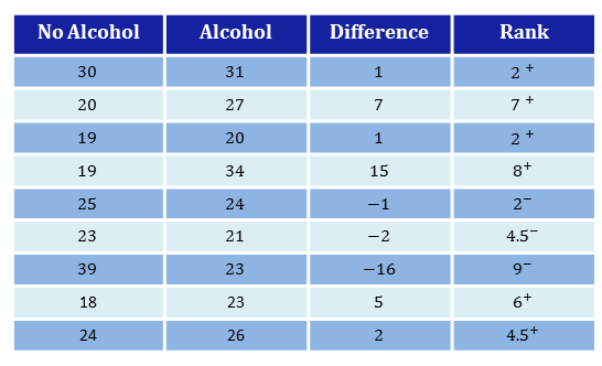
We already calculated the differences in the Sign test example, so now we just need to assign the ranks and attach the signs as superscripts.
|center
To calculate the rank of $1$ we first count up the number of $1$'s in the table (both $+1$ and $-1$ are included in this). We find that there are $3$. So the rank of these becomes $\dfrac{1+2+3}{3}=2$ as there are three $1$'s so they take the average value of the three individual ranks. Then we attach the signs as superscripts. Hence the rank of $+1$ is $2^+$ and the rank of $-1$ is $2^-$.
The sum of the positive ranks is: $2 + 7 + 2 + 8 + 6 + 4.5 = 29.5$.
The sum of the negative ranks is: $2 + 9 + 4.5 = 15.5$.
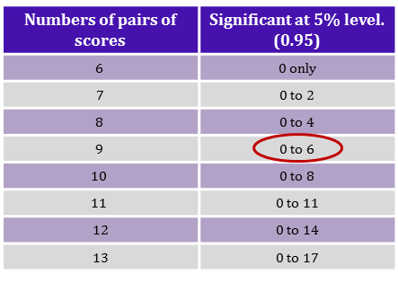
Here the smaller sum of ranks is $T = 15.5$, which we compare to a significance table.
|center
Since $11$ does not lie in the range $0 - 6$, we can conclude that our value is not statistically significant. There is no evidence to suggest here that alcohol has an effect on reaction time, we accept the null hypothesis. Once again, these results suggest more experiments should be carried out with changes to the experimental design, such as using more participants or increasing the units of alcohol.
An accurate report of our findings would be:
'The reaction times for the alcohol group $(\bar{X} = 25.444)$ (3 d.p.) were slower than for the no alcohol group $(\bar{X}=24.111)$ (3 d.p.). However, this difference was insufficient; so we cannot reject the null hypothesis that alcohol has no effect on reaction times $(T = 11, n =9, p >0.05,$ ns$)$.
Note: ns means not significant.