Continuous Probability Distributions (Business)

This is a subject-specific page for Business 2 students.

The Probability Density Function

Since a continuous random variable can take any value within its range, we cannot list all the possible values and their probabilities as in the discrete case. For instance the rate of inflation could be recorded to any number of decimal places so it is impossible to list all possible inflation rates.

For continuous random variables we represent probabilities using a probability density function (pdf) (sometimes just called the probability distribution). The pdf of a continuous random variable $X$, is a function $f(x)$ defined such that:

• Its curve lies on or above the $x$-axis, i.e. $f(x) \ge 0$ for all $x$ in its range.
• The area under the entire curve is $1$.
• The probability $\mathrm{P}(a<X<b)$ that $X$ lies between $a$ and $b$ is the area under the curve between $a$ and $b$.

Below is an example of what a pdf might look like. The region shaded green is $\mathrm{P}(2 \leq X \leq 3)$. The total shaded area (purple and green) is equal to $1$.

Cumulative Probabilities

As for discrete random variables, if $X$ is a random variable then the cumulative probability ($P(X \leq 10)$ for example) is the probability that $X$ takes any value less than or equal to $10$.

The cumulative distribution function (cdf) gives the probability that the random variable $X$ is less than or equal to $x$ (i.e the cumulative probability) and is usually denoted $F(x)$. It is equal to the area under the curve of the pdf $f(x)$.

The Expected Value and Variance

In general, calculating the expected value (mean) and variance of a continuous random variable requires using integration (not covered here). However, the continuous probability distributions you will be dealing with in this section have well known formulae for the means and variances and we use these formulae.

Normal Distribution

The Normal distribution is the most widely used and frequently occurring continuous probability distribution.

The formula for the pdf of the Normal distribution is:

where $\mu$, the mean and $\sigma^2$ is the variance (the square of the standard deviation, $\sigma$)

If a random variable $X$ follows a Normal distribution we write $X$~$\mathrm{N}(\mu, \sigma^2)$

An example of the Normal distribution in Business

Suppose that the owner of a company selling climbing equipment already sells climbing helmets for children but wants to start selling helmets for adults as well.The company plans to sell separate helmets for men and for women and wants to know how many of each size (small, medium or large for male and female separately) to produce. The company may assume that a person's head size approximately follows a Normal distribution with a separate mean and variance for males and females So, using the Normal distribution as a model, the owner can order the appropriate numbers and sizes of helmets.

What does the Normal distribution look like?

The probability density function (pdf) for a Normal random variable is bell-shaped and is symmetric about the mean value, $\mu$. In the plot below $\mu=0$. Although the plot only shows the curve in the range $-5 \leq X \leq +5$, the curve goes all the way out to minus infinity and plus infinity.

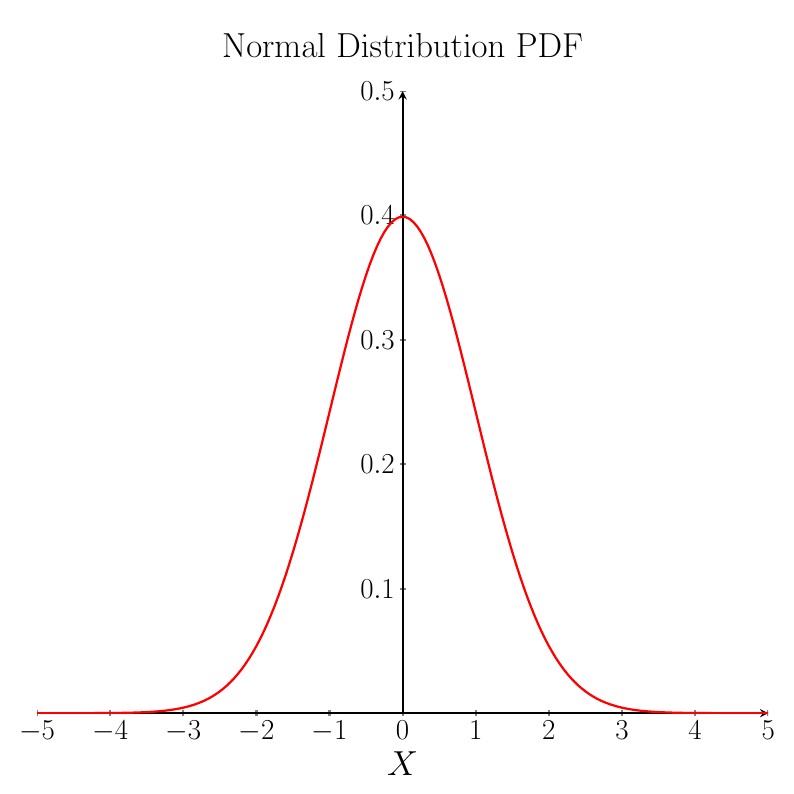
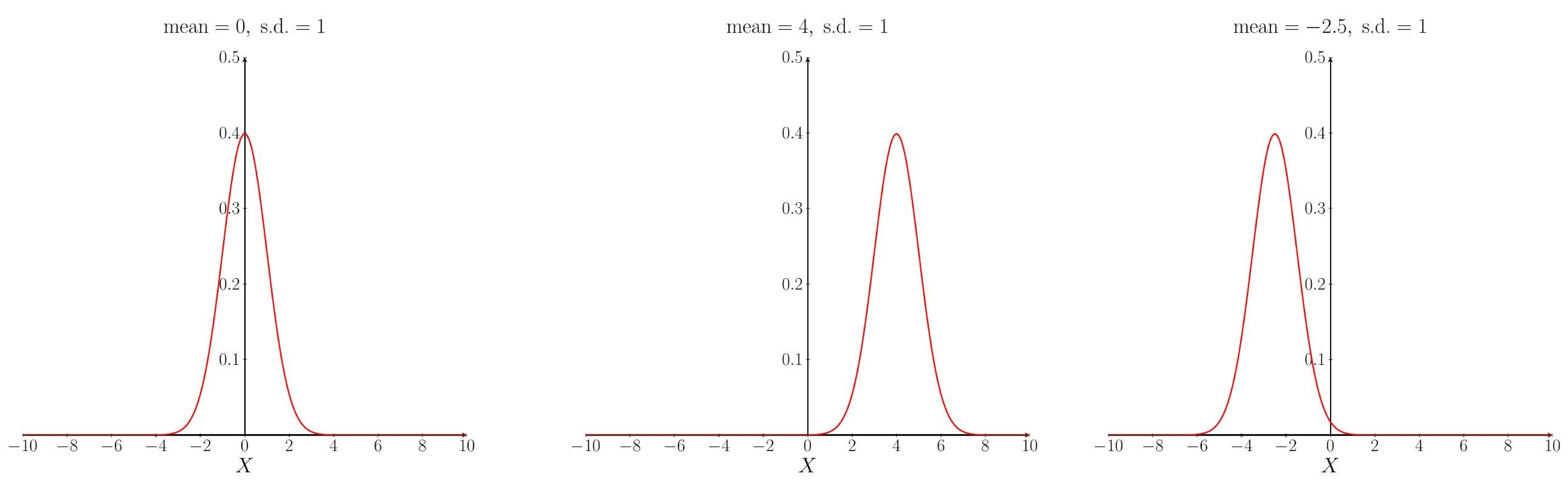
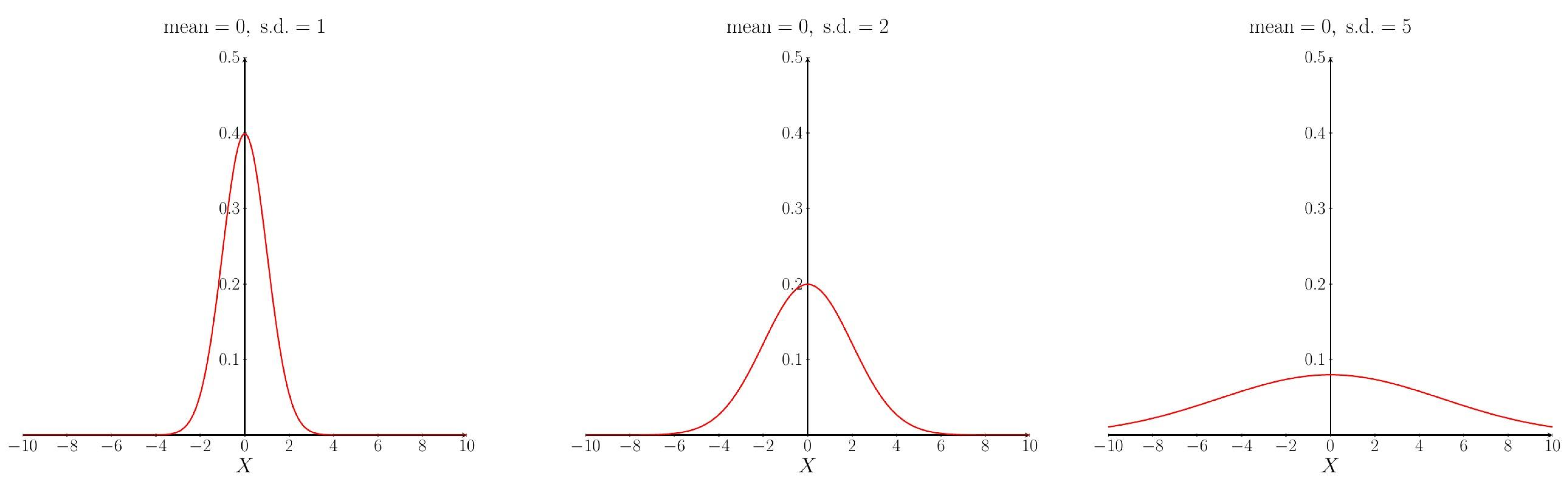
The shape of the pdf curve depends upon the values of the parameters $\mu$ and $\sigma$. Changing the mean $\mu$ affects the location (on the $X$-axis) of the peak of the curve: increasing the mean moves the curve to the right, decreasing the mean moves the curve to the left. The standard deviation $\sigma$ determines how spread out the curve is: increasing the standard deviation makes the curve more spread out and decreasing the standard deviation makes the curve narrower.

Calculating Probabilities

Suppose we have a random variable $X$ which follows a Normal distribution with mean $0$ and standard deviation (s.d.) $1$.

$\mathrm{P}(0 \leq X \leq 1)$ is equal to the area of the shaded region on the graph shown below.

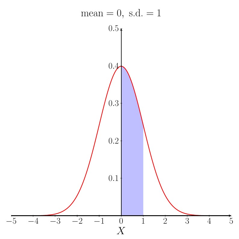
These probabilities are found by looking up standard Normal distribution tables or you can use computer packages, such as R and Minitab, to find them. For more detailed information about the Normal distribution, including how to look up probabilities in tables, click here. From the tables, we find that the shaded area above is equal to $0.3413$.

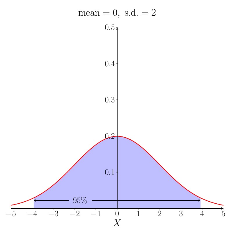
$95\%$ of the area under the Normal distribution $\mathrm{N}(\mu,\sigma^2)$ pdf curve lies in the range $\mu- 1.96 \times \sigma \leq X \leq \mu+ 1.96 \times \sigma$.

A good way to remember this is that $95\%$ of the area under the curve lies within roughly $2$ standard deviations of the mean. The figure below shows the case when the mean is $0$ and the s.d. is $2$.

Standardising

A Standard Normal distribution has $\mu = 0$ and $\sigma = 1$. A non-standard Normal random variable $X$, which has mean $\mu \neq 0$ and/or standard deviation $\sigma \neq 1$ can be standardised as follows:

Take $X$, the variable, and subtract its mean $\mu$, then divide by its standard deviation $\sigma$. We then call the result $Z$.

We then can compute probabilities using $Z$ and standard Normal tables.

Example 1

The owner of Fredds, a chain of popular bakery stores in the North East, supplies all of her employees with a uniform. She is ordering a bundle of uniforms for new employees hired within the next year and needs to decide what sizes and how many uniforms of each size to buy. The only difference between uniforms is their height and the owner assumes that peoples' heights follow a Normal distribution with $\mu = 170$cm and $\sigma^2 = 49$cm. Calculate the probability that a randomly selected (future) employee is:

(A) Smaller than 160cm.

(B) Between 165cm and 175cm.

(C) Taller than 185cm.

Solutions

Here, we have a Normal random variable, $X$~$\mathrm{N}(170,49)$. Firstly, we need to standardise $X$ to $Z$ where $\mu = 170$, $\sigma = \sqrt{49} = 7$. So, \begin{align} Z &= \dfrac{X-\mu}{\sigma}\\ &= \dfrac{X - 170}{7}\\ \end{align}.

Solution (A)

To find the probability that a randomly selected employee is smaller than 160cm, we first write: \begin{align} \mathrm{P}(X&<160).\\ \end{align}

Then standardise both sides of the inequality.

\begin{align} & \; \; \; \; \; \; \mathrm{P}\left (\dfrac{X - 170}{7} < \dfrac{160 - 170}{7} \right)\\ &\Rightarrow \mathrm{P} \left (Z< \dfrac{160 - 170}{7} \right)\\ &= \mathrm{P}(Z< -1.43)\;\;\text{ (to 2 d.p)}\\ \end{align}.

We then need to look up $Z=-1.43$ in a $Z$-table to find the corresponding probability.

We find that the probability is $0.0764$. So, \begin{align} &\; \; \; \; \; \; \mathrm{P}(Z < -1.43) = 0.076 \text{ (to 3 d.p)}\\ &\Rightarrow \mathrm{P}(X< 160) = 0.076.\\ \end{align}

Solution (B)

Now we require the probability that a randomly selected employee is taller than 165cm but smaller than 175cm. That is, we require

\begin{align} &\mathrm{P}(165Finally, we require:

The Uniform Distribution is another important distribution. If the random variable $X$ follows a uniform distribution then we write $X \text{~} \mathrm{U}(a,b)$ where $a$ and $b$ are the parameters of the distribution and:

• $a$ is the lowest value that $X$ can take.
• $b$ is the highest value that $X$ can take.

Hence $a \le X \le b$

The only restriction on the values of these parameters is that $b>a$..

The important characteristic of the Uniform Distribution is that is has a constant probability. That is, all values of X in the range from $a$ to $b$ are equally likely.

The formula for the probability density is:

The formula for the cumulative probability is:

The expectation and variance of a Uniform random variable are:

What does a Uniform Distribution look like?

Below is a plot of the probability density function (pdf) for a $\mathrm{U} (3,16)$ Distribution. The entire shaded area (blue and grey) is equal to $1$. The blue areas represent $\mathrm{P}(5 \leq x \leq 7)$ and $\mathrm{P}(10 \leq x \leq 12)$ and we can see that the areas are the same and so the intervals have the same probabilities.

Example 2

A local authority is responsible for a stretch of road $4$km long in Gerrards Cross. Elderly residents of this road have been complaining of the distance to the nearest post box for a long time and The Postal Service have finally agreed to install a post box on this stretch of road but have no yet specified exactly where. The local authority assumes that all locations along this stretch of road are equally likely to have been chose by The Postal Service.

Let $Y$ be the distance along the road (from the East end of the road) where the new post box will be installed.

(A) What distribution does $Y$ follow? And what is the expectation and variance?

'''(B) The pavement on either side of the stretch of road becomes very narrow between $1$ and $1.01$ kilometres from the East of the road. The Local Authority is concerned about the possibility of the new post box being installed in this section of the road as it would make the pavement even narrower and people will not be able to get past with wheelchairs or prams. What is the probability of the post box being installed in this section of road according to the beliefs of the Local Authority?

Solutions

Solution (A)

Since we are considering this problem from the point of view of the Local Authority we have no prior knowledge of where the post box will be installed and so the Uniform Distribution is appropriate (all locations are equally likely from the Local Authority's perspective). Here the minimum and maximum values are given by $a = 0$ and $b = 4$ so we have:

\begin{align} Y \text{~} \mathrm{U}(0,4),\\ \end{align} The expected value of $Y$ is: \begin{align} \mathrm{E}[Y] &= \dfrac{0+4}{2}\\ &= 2.\\ \end{align} The variance is: \begin{align} \mathrm{Var}(Y)&=\dfrac{(4-0)^2}{12}\\ &=\dfrac{16}{12}\\ &=\dfrac{4}{3}.\\ \end{align}

Solution (B)

We wish to calculate $\mathrm{P}(1\leq Y \leq 1.5)$. We can do so using the formula in the second blue box above. \begin{align} \mathrm{P}(1\leq Y \leq 1.5) &= \mathrm{P}(X \leq 1.5) - \mathrm{P}(X \leq 1)\\ &=\dfrac{1.5-0}{4-0} - \dfrac{1-0}{4-0}\\ &=\dfrac{1.5}{4}-\dfrac{1}{4}\\ &=\dfrac{0.5}{4}\\ &=\dfrac{1}{8}\\ &= 0.125.\\ \end{align}

So there is a $0.125$ chance the post box will be installed along the stretch of road with narrow pavements according to the beliefs of the Local Authority.

Exponential Distribution

The Exponential Distribution is another important distribution and is typically used to model times between events or arrivals.The distribution has one parameter, $\lambda$ which is assumed to be the average rate of arrivals or occurrences of an event in a given time interval.

If the random variable $X$ follows an Exponential distribution then we write: $X \text{~}\mathrm{Exp}(\lambda)$.

The probability density function is:

(Cumulative) probabilities can be calculated using:

The expectation and variance for an Exponential random variable are:

An example of the Exponential distribution in Business

It is assumed that the average time customers spends on hold when contacting a gas company's call centre is five minutes. The company has a policy that if a customer waits for longer than $15$ minutes they are entitled to claim $£5$ off their next quarterly bill.

If the company employs a new team, at some expense,then the average waiting time is reduced to four minutes.

The director of the company must decide whether or not to employ a new team. He thinks the idea is only worthwhile if the probability that a customer waits for longer than $15$ minutes is reduced by at least $0.025$.

This situation can be modelled using Exponential distributions: one for waiting times (times on hold) under the current team and one for waiting times under a new team.

With the current team the mean waiting time is $5$ minutes and so the mean rate of calls answered per minute is given by $\lambda_1=1/5=0.2$. The corresponding Exponential distribution is $\mathrm{Exp}(0.2)$.

Similarly, with a new team, we have $\lambda_2=1/4=0.25$ and so the corresponding Exponential distribution is $\mathrm{Exp}(0.25)$.

Determine whether the director should employ a new team or keep his current team.

Solution

Let $X$ denote the waiting time of a customer under the current team. We know that $X$ follows an Exponential distribution with parameter $\lambda_1=0.2$ so we have $X\sim Exp(0.2)$. Now we need to calculate $P(X>15)$.

\begin{align} \mathrm{P}(X > 15) &= 1 - \mathrm{P}(X \leq 15)\\ &= 1 - \big(1 - e^{-0.2 \times 15}\big)\\ &= e^{-3}\\ &= 0.050 \text{ (to 3 d.p.)}. \end{align}

So the probability that a customer waits for longer than 15 minutes is 0.050 (to 3 d.p.).

Now we consider the probability of this event under a new team. Let $Y$ denote the time a customer waits under a new team $Y\sim Exp(0.25)$. We know that $Y$ follows an Exponential distribution with parameter $\lambda_2=0.25$ so we have $Y\sim Exp(0.25)$. Thus,

\begin{align} \mathrm{P}(Y > 15) &= 1 - \mathrm{P}(Y \leq 15)\\ &= 1 - \big(1 - e^{-0.25 \times 15}\big)\\ &= e^{-3.75}\\ &=0.024 \text{ (to 3 d.p.)}. \end{align}

Recall that the director of the company would only opt for recruiting a new team if the probability that a customer waits longer than 15 minutes is reduced by at least 0.025.

\begin{align} \text{Change in probability} &= \text{Probability without a new team} - \text{Probability with a new team}\\ &= e^{-3} - e^{-3.75}\\ &= 0.026 \text{ (to 3 d.p.)}.\\ \end{align}

Since $0.026>0.025$, the director of the company should recruit a new team.

What does an Exponential distribution look like?

Below are some examples of what the pdf for various exponential distributions look like.

Example 3

The time in minutes, $X$, between the arrival of successive customers at a post office is exponentially distributed with pdf $f(x) = 0.2 e^{-0.2x}$.

(A) What is the expected time between arrivals?

(B) A customer walks into the post office at $12.30$p.m. What is the probability the next customer arrives:

(i) on or before $12:32$p.m.?

(ii) after $12:35$p.m.?

Solutions

Solution (A)

Here $\lambda = 0.2$ and so the mean time between arrivals is $\frac{1}{0.2} = 5$ minutes.

Solution (B)

(I) If the next customer arrives on or before $12:32$p.m., it means that the time between their arrival and the previous arrival is at most $2$ minutes. So, we require $\mathrm{P}(X \leq 2)$.

Using the formula above we have:

\begin{align} \mathrm{P}(X \leq 2) &= 1 - e^{-0.2 \times 2}\\ &= 1 - 0.67032\\ &= 0.330 \text{ (to 3 d.p.)}\\ \end{align}

(ii) If the next customer arrives after $12:35$ p.m. then the time between the two customers is more than $5$ minutes. We now require $\mathrm{P}(X>5)$. To calculate $\mathrm{P}(X>x)$. This is equivalent to $1 - \mathrm{P}(X \leq x)$ and so:

\begin{align} \mathrm{P}(X > 5) &= 1 - \mathrm{P}(X \leq 5)\\ &= 1 - (1 - e^{-0.2 \times 5})\\ &= e^{-1}\\ &= 0.368 \text{ (to 3 d.p.)}.\\ \end{align}.

Poisson Processes

The Exponential distribution is often used as a model for the times between events. We have looked at events occurring randomly in time in association with the Poisson distribution. The Poisson distribution gives the probabilities for the number of events taking place in the given time period whereas the exponential distribution gives the probabilities for times between the events. Both of these concern events occurring randomly in time at a constant average rate, $\lambda$. This is known as a Poisson process.

For example, consider a series of randomly occurring events, such as customers entering a bank. The times of arrivals might look like this:

.

There are two ways we can view the data.

1. The number of arrivals in each minute ($1, 1, 0, 3, 1$).
2. The times between successive arrivals.

For the Poisson process we have,

• the number of arrivals follows a Poisson distribution with parameter $\lambda$, and

• the time between successive calls has an exponential distribution with parameter $\lambda$.

Other Continuous Probability Distributions

There are other important continuous probability distributions which you will meet in practical business problems and decision making. In particular, you will meet the Student's t-distribution or t distribution and the Chi-squared ($\chi^2$) distribution. The t-distribution is used when testing a hypothesis about a mean or a difference between two means. The Chi-squared distribution is used when analysing categorical data.

Test Yourself

Click on the following links to practise Numbas tests on the distributions on this page:

Test yourself: Numbas test on calculating probabilities from a normal distribution

Test yourself: Numbas test on the exponential distribution and uniform distribution