Introduction to Probability (Business)

This is a subject-specific page for Business 2 students.

Background Information

Definitions

Experiment - An activity where we do not know for certain what will happen, but we will observe what happens, e.g. we roll a fair die.

Outcome- One of the possible things that can happen, e.g. we roll a six.

Event - A particular collection of outcomes e.g. we roll an even number: there are 3 possible outcomes in this event (we could roll a two, a four or a six).

Sample Space - The set of all possible outcomes, e.g. we can roll a one, two, three, four, five or six.

Mutually Exclusive - Two events are mutually exclusive if both cannot occur at the same time, for example, we cannot roll a six and an odd number at the same time.

Independent - Two events are independent if the occurence of one does not affect the probability of the other occuring, e.g. rolling a 6 the first time does not affect the probability of rolling a 6 the next time.

What is probability?

Probability is a mathematical way of describing how likely an outcome or event is to occur. Probabilities are usually expressed as fractions, decimal numbers or percentages and are measured on a scaled between zero and one. An impossible event has a probability of zero and a certain event has a probability of one.

Notation

$S = \{...\}$ is the sample space, e.g. $S = \{1, 2, 3, 4, 5, 6\}$ for rolling a fair die.

$\mathrm{P}(\text{event})$ means the probability of the event occuring.

Illustrative Example

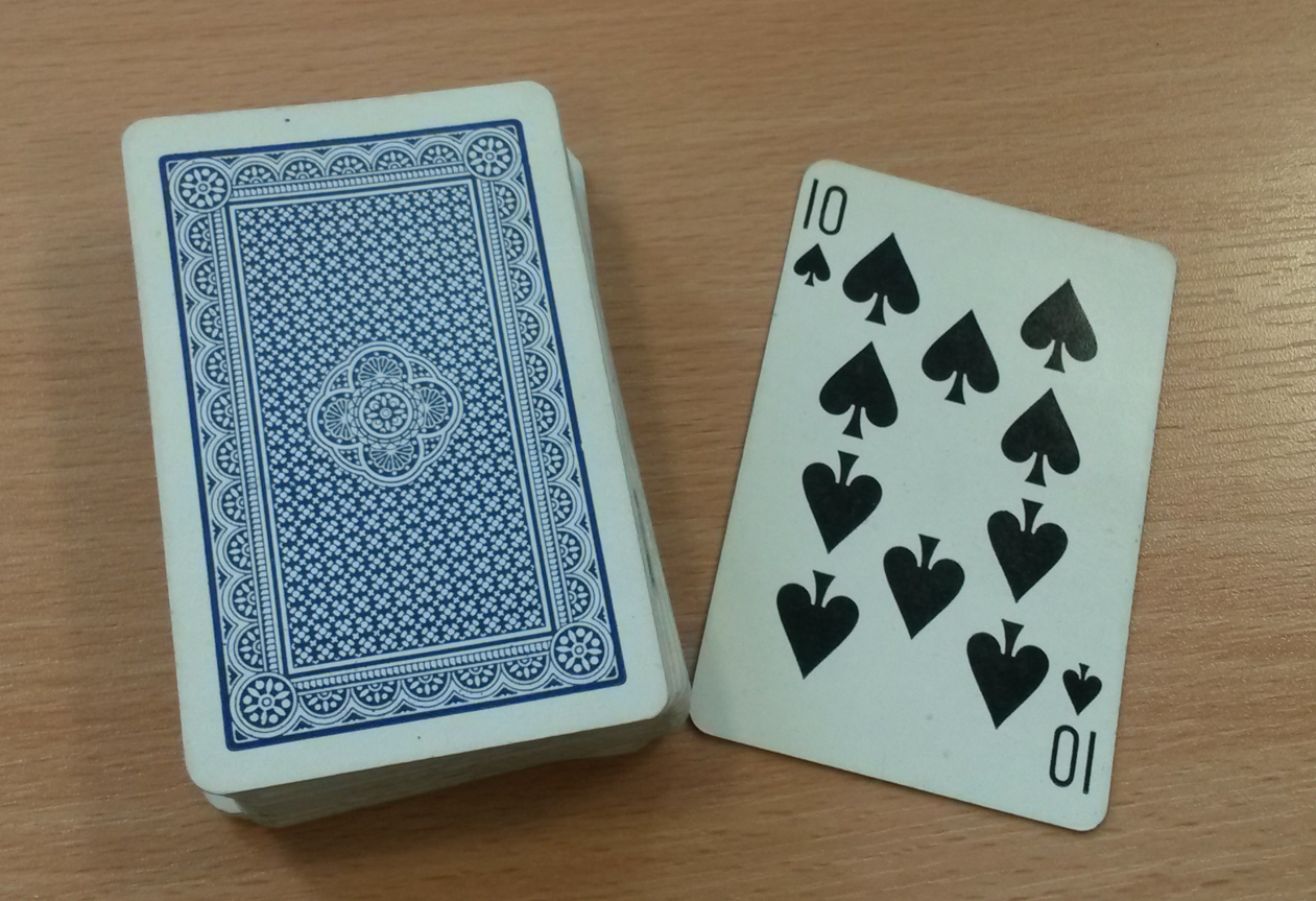
Suppose we have an ordinary deck of $52$ playing cards (without the jokers) and we draw one card from the deck at random and then look to see what card we have drawn. The experiment is the act of drawing a card from the deck, the outcome is the particular card that we happen to draw, and the sample space is the set (collection) of all the different cards in the deck.

There are lots of different possibilities for events, here are just a few:

1) We draw a red card (hearts or diamonds). There are $26$ outcomes in this event so the probability of this event is: \begin{align} P(\text{red card})=\dfrac{26}{52}\\

0.5 \end{align}. 2) We draw an ace. There are $4$ outcomes in this event so the probability of this event is: \begin{align} P(\text{ace})\\

0.08 \text{ (to 2 d.p.)} \end{align}. 3) We draw the $10$ of spades. There is just one outcome in this event.

4) We draw a red card which is also an ace. There are $2$ outcomes in this event.

5) We draw a card that is black and a diamond. There are $0$ outcomes in this event.

6) We draw a card that is red or black. There are $52$ outcomes in this event.

Event $5$ is an example of an impossible event, it cannot happen. Black cards are either clubs or spades but not diamonds. Notice that there are zero outcomes in this event. Even though this cannot ever happen, we still call this an event.

Event $6$ is an example of a certain event, it must happen. Whatever card we draw it must be either red or black. Notice that every outcome in the sample space (every one of the $52$ cards in the deck) is in this event.

Events $2$ and $3$ are mutually exclusive. Either of them can occur but not both at the same time, if we draw an ace then we cannot also have drawn the $10$ of spades (we are only drawing one card) and vice versa.

Events $1$ and $2$ are independent. If we draw a red card this does not affect the probability that the card is an ace. Similarly, if we draw an ace, this does not affect the probability that the card is red.

Laws of Probability

The following two laws will be useful when carrying out probability calculations:

Multiplication Law - The probability of two independent events $A$ and $B$ both occurring at the same time can be written as:

Addition Law - The probability that either event $A$ or event $B$ will happen is given by:

Examples

Example 1

In Newcastle, $70\%$ of small businesses use the internet to advertise new products; $50\%$ of small businesses use flyers to advertise new products and a quarter of small businesses use both flyers and the internet.

(A) What is the probability that a randomly chosen small business in Newcastle uses either flyers or the internet to advertise new products?

(B) What is the proportion of small businesses in Newcastle that use neither the internet nor flyers to advertise new products?

Solution (A)

• Let $F$ denote the event that a business advertises new products using flyers and $I$ denote the event that a business uses the internet to advertise new products.

• We wish to find $\mathrm{P}(F \; \text{or} \; I)$. Using the Addition Law, we have:

\begin{align} \mathrm{P}(F \; \text{or} \; I) &= \mathrm{P}(F) + \mathrm{P}(I) - \mathrm{P}(F \; \text{and} \; I)\\ &= \frac{7}{10} + \frac{1}{2} - \frac{1}{4}\\ &= \frac{19}{20} = 0.95.\\ \end{align}

• There is a $95\%$ probability that a randomly chosen business in Newcastle uses either flyers or the internet to advertise new products.

Solution (B)

We use the solution to part (A) to answer this question. In part (A) we found the proportion of firms that use either the internet or flyers or both the internet and flyers to advertise new products. The proportion of small businesses in Newcastle that use neither the internet nor flyers to advertise new products is the only remaining event and is therefore calculated as:

\begin{align} 1 - \mathrm{P}(F \; \text{or} \; I) &= 1 - \dfrac{19}{20}\\ &= \dfrac{1}{20} = 0.05.\\ \end{align}

So one out of twenty (or $5\%$ of) small businesses in Newcastle use neither advertising method.

Example 2

$60\%$ of employees at a department store in Newcastle are women. Government research into methods of commuting to city jobs in the North East has shown on average that:$ \;$

• $12\%$ of people cycle into work.
• A quarter of the people drive.
• $10\%$ of people walk.
• And the rest use public transport.

What is the probability that a randomly selected employee of the department store in Newcastle commutes using public transport and is male?

Solution

Since gender and method of commuting are independent in this example we can use the Multiplication Law.

First we need to calculate the probability that a person uses public transport to commute, which we shall denote as $P(T)$. \begin{align} \mathrm{P}(T) &= 1 - \mathrm{P}(\text{Not} \; T)\\ &= 1 - (0.12+0.25+0.1)\\ &= 0.53.\\ \end{align}

We then let $M$ denote the event that the randomly selected employee is male.

So the probability that a randomly selected employee is a male who commutes using public transport is: $\; $

\begin{align} \mathrm{P}(M \; \text{and} \; T) &= \mathrm{P}(M) \times \mathrm{P}(T)\\ &= 0.4 \times 0.53\\ &= 0.212.\\ \end{align}

Conditional Probability

What is conditional probability?

When events are not independent we must use conditional probability. The conditional probability of A occurring given B is the probability of event A occurring given that event B has already taken place and is denoted \[\mathrm{P}(B|A)\].

We can use this conditional probability, with the multiplication law, to give:

or

Example 3

$70\%$ of households in Newcastle watch the news on an evening and $50\%$ of households watch the news on both the evening and in the morning. What is the probability that a household, which watches the news in the evening, will also watch the morning news?

Solution

First we denote by $E$ the event that the household watches the news on the evening and $M$ the event that the household watches the morning news.

From the question we have $\mathrm{P}(E) = 0.7$ and $\mathrm{P}(E \; \text{and} \; M) = 0.5$.

We want to calculate $\mathrm{P}(M|E)$.

We can use and rearrange the equation of the multiplication law in the blue box above as follows:

\begin{equation} \begin{split} \mathrm{P}(E \; \text{and} \; M) &&= \mathrm{P}(E) \times \mathrm{P}(M|E)\\ \mathrm{P}(M|E) &&= \dfrac{\mathrm{P}(E \; \text{and} \; M)}{\mathrm{P}(E)}\\ \end{split} \end{equation} Inserting the values of these probabilities given above into this equation gives:

\begin{align} \mathrm{P}(M|E) &= \dfrac{0.5}{0.7}\\ &=\dfrac{5}{7}\\ &= 0.714\text{ (to 3 d.p).}\\ \end{align}

The probability that a household that watches the news on the evening also watches the morning news is $\dfrac{5}{7} = 0.714\text{ (to 3 d.p).}$

Decision Making using Probability

Expected Monetary Value

The Expected Monetary Value $(\mathrm{EMV})$ of a single event is calculated as the sum of the monetary value of each outcome in that event multiplied by its probability. That is,

where the sum is over all possible outcomes in the event.

Tree Diagrams

Tree Diagrams can be used to help us to visualise and calculate complex probabilities. When drawing a tree diagram we begin with a dot. From this dot lines (“branches”) are then drawn, extending from the right of the first dot, to represent all possible outcomes for the given situation. The probabilities of each of these outcomes is written just above the corresponding line.

To calculate the probability that two events both happen, we draw another “branch” extending from the “branch” corresponding to one of these events to represent the second event occurring after the first. Above this line we write the probability (or conditional probability for events which are not independent) of the second event occurring after the first. Multiplying these probabilities “along the branches” gives the required probability.

To calculate the probability that one or both of two independent events occurs we add the probabilities of the two events “down the columns”.

The following example illustrates this idea:

An Example of using a Tree Diagram

Consider Example 2 again. Now calculate the probability that a randomly selected employee is female and drives into work.

Solution We can use a tree diagram to present all of the information given to us and calculate the required probability.

The probabilities in blue are calculated using the multiplication law. So, the probability the employee is female and drives is $0.6 \times 0.25 = 0.15$.

Tip: To make sure all your calculations are correct, you can check to see that your final probabilities (the blues ones) add up to $1$. This must be the case because at least one of all of the possible events must (is certain to) occur.

Decision Trees

Decision trees are very similar to the probability tree diagrams but are used specifically to calculate expected monetary values.

Example 4

The manager of a small business has the opportunity to buy a fixed quantity of a new product and offer it for sale for a limited time.

There will be a fixed cost of $£100,000$ to buy the product and offer it for sale. The amount of the product that the manager would be able to sell is not certain but market research has suggested that:

• The probability that sales would be “poor” is $0.25$. Selling this quantity would raise an income of $£75,000$.
• The probability that sales would be “medium” is $0.6$. Selling this quantity would raise an income of $£110,000$.

• The probability that sales would be “good” is $0.15$. Selling this quantity would raise an income of $£145,000$.

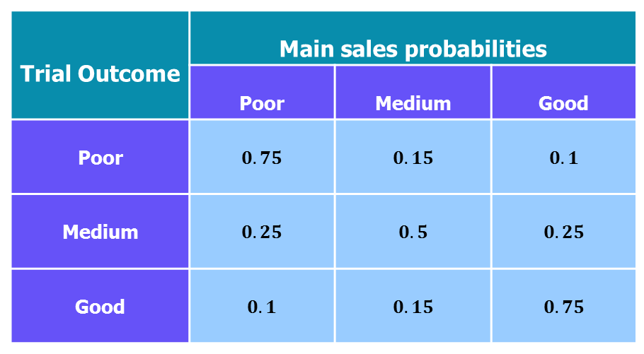
The product can be sold for a trial period before a final decision is made and it costs $£18,000$ to run the trial. The results of the trial will be “poor” with probability $0.35$, “medium” with probability $0.4$ or “good” with probability $0.25$. Knowing the outcome of the trial changes the probabilities for the main sales project:

The manager will make decisions based on expected monetary value.

(A) Draw a decision tree for this problem.

(B) What is the $\mathrm{EMV}$ of a decision to go ahead with the product without a trial?

(C) Complete the solution of the decision problem and determine the optimal course of action for the company.

Solution (A)

The values in the blue boxes are the final incomes from buying the new product when sales are “poor”, “medium” or “good” (top to bottom).

Solution (B)

To calculate the expected monetary value we need to utilise the formula in the pink box above.

• For No Trial:

\begin{align} \mathrm{EMV} &= 0.25 \times £75,000 + 0.6 \times £110,000 + 0.15 \times £145,000\\ &=£106,500.\\ \end{align}

The manager has an expected income of $£106,500$ from selling the new product without a trial.

Solution (C)

To solve the decision problem it is best to first calculate the seperate $\mathrm{EMV}$s for when a trial is run and when a trial is not run. We must then compare the $\mathrm{EMV}$s for each option (trial or no trial) and choose the option with the highest $\mathrm{EMV}$. This is the optimal course of action for the company.

• When a trial is carried out and has a poor result:

\begin{align} \mathrm{EMV} &= 0.75 \times £75,000 + 0.15 \times £110,000 + 0.1 \times £145,000\\ &=£87,250.\\ \end{align}

• When a trial is carried out and has a medium result:

\begin{align} \mathrm{EMV} &= 0.25 \times £75,000 + 0.5 \times £110,000 + 0.25 \times £145,000\\ &=£110,000.\\ \end{align}

• When a trial is carried out and has a good result:

\begin{align} \mathrm{EMV} &= 0.1 \times £75,000 + 0.15 \times £110,000 + 0.75 \times £145,000\\ &=£132,750.\\ \end{align}

Now to calculate the overall $\mathrm{EMV}$ we multiply each of these by their associated probabilities: \begin{align} \mathrm{EMV} &= \mathrm{P}(\text{Poor result}) \times £87,250 + \mathrm{P}(\text{Medium result)} \times £110,000 + \mathrm{P}(\text{Good result}) \times £132,750\\ &=£107,725. \end{align}

We now need to calculate the expected profit (or loss) the business would make from each option (trial or no trial).

• No Trial: \begin{align}

\text{Expected Profit} &= \mathrm{EMV} \text{ for no trial} - \text{Cost of new product}\\ &=£106,500 - £100,000\\ &=£6,500. \end{align}

So if the manager goes ahead with the product without a trial, the expected profit is $£6,500$.

• Trial: \begin{align}

\text{Expected Profit} &= \mathrm{EMV}\text{ for trial} - \text{Cost of new product} - \text{Cost of trial}\\ &=£107,725 - £100,000 - £18,000\\ &=-£10,275. \end{align}

With the trial, there will be an expected loss of £10,275.

From these results we can see that optimal course of action for the company is to sell the new product but without the trial period as this yields a higher $\mathrm{EMV}$. It is important to note that although the expected monetary value is higher when the manager chooses not to run the trial, the realised profit or loss may be or may not be better than it would have been if a trial had been carried out.

Probability Distribution Definitions

Variable - A variable is a quantity which we do not yet know the value of and is denoted by a lower case letter e.g. total number of sales this week at a newsagent, gender of an employee, the annual rate of inflation etc.

Random Variable - A variable whose value depends on the outcome of an experiment. For example, our variable could be the outcome of flipping a coin. There are two outcomes, heads or tails, and the probability for each outcome is $\dfrac{1}{2}$.

Note: Capital letters $X$, $X_1$, $X_2$, $Y$ etc. are used to denote random variables, and lower case letters $x$, $x_1$, $x_2$, $y$ etc. are used to denote the corresponding values (i.e., the actual values that the random variables take).

Discrete Random Variable - A variable which can take one of a countable set of values within a specified range. Examples include the number of students present in a class (a student can't be half present!), a student's grade level, prices etc..

Continuous - A random variable which can take any value (not just whole numbers) within a given range, e.g. annual rate of inflation, the height of a student, time etc..

Probability Distribution - A probability distributions tell us all the values a random variable can take, along with their associated probabilities. A probability distribution can be presented as an equation, a chart or a table. For any probability distribution, the sum of the probabilities of all mutually exclusive events is always one.

Expectation - The average (mean) value of a random variable. Or more formally, the value of a random variable we would “expect” to see if we repeated the random variable process a very large number of times.

Variance - The variance tells us how spread out the values of the outcomes of an experiment are. Equivalently, it tells us how far away, on average, the values of the outcomes of an experiment are from the mean value. A large variance indicates that the values will very spread out, whereas a small one suggests the values lie close to the mean.

Test Yourself

Test yourself: Probability

See Also

To develop these ideas further see discrete probability models and continuous distributions.