Numeracy, Maths and Statistics - Academic Skills Kit

T-Test

ContentsToggle Main Menu 1 t-tests - Population variance unknown1.1 One Sample t-tests1.2 Two Sample t-tests 2 The t-table 3 Worked Examples 4 Test Yourself 5 See Also

This is a subject-specific page for Psychology students.

t-tests - Population variance unknown

The t-test is very similar to a $z$-test, however, you do not know the value of the population variance $\sigma^2$ and so you must use a modified version of the test above.

One Sample t-tests

This is where you are only testing one sample, for example, the number of patients currently being treated with Cognitive Behavioural Therapy at a clinic. Usually you would compare your data with a known value, typically a mean that has often been previously derived from other research. You want to test the null hypothesis i.e. is the mean of the sample the same as the known mean?

The Method

The first two steps for a t-test are the same as for a $z$-test, as we must identify the null and alternative hypothesis.
Now we calculate the test statistic using the below formula, as you can see there are only slight changes. It is now labelled t and the population variance has been replaced by the sample variance.

\begin{equation} t = \dfrac{\bar{x}-\mu}{\sqrt{\dfrac{s^2}{n}}} \end{equation}

Now you use t-tables (see below) to find the $10$%, $5$% and $1$% critical values at the correct degrees of freedom ($n-1$) and compare our t-statistic.
Make conclusions. If your t-statistic is greater than any of these values we have a significant result at that level, meaning you can reject the null hypothesis, and if not accept it.

See the worked example below.

Two Sample t-tests

A two sample t-test compares two samples of normally distributed data. We shall look at two types of two sample t-tests:

Paired t-test/related t-test - comparing two sets of results where they are linked (where you test the same group of participants twice or your two groups are similar). See worked example later.
Independent/unrelated t-test - there is no link between the groups (different independent groups).

The main difference between these two tests is that the t-statistic is calculated differently.

For paired/related t-tests the t-statistic is:

\begin{equation} t = \dfrac{\bar{d}}{\sqrt{\dfrac{s^2}{n}}} \end{equation}

where $\bar{d} $is the mean of the differences between the samples. You will compare the t-statistic to the critical values in a t-table on $(n - 1)$ degrees of freedom. Here $s$ is the standard deviation of the differences.

Whereas for the unrelated t-test, the test statistic is:

\begin{equation} t = \dfrac{\bar{x_1} - \bar{x_2}}{\sqrt{s^2\bigg(\dfrac{1}{n_1} + \dfrac{1}{n_2}\bigg)}} \end{equation}

where the pooled standard deviation $s$ is:

\begin{equation} s =\sqrt{\dfrac{(n_1 - 1)s_1^2 + (n_2 - 1)s_2^2}{n_1 +n_2 -2}} \end{equation}

where $\bar{x_1}$ and $\bar{x_2}$ are the means from the two samples, likewise $n_1$ and $n _2$ are the sample sizes and $s_1^2 \text{and } s_2^2$ are the sample variances. This test statistic you will compare to t-tables on $(n_1 + n_2 - 2)$ degrees of freedom.

Note: for the pooled variance t-test to be appropriate you rely on the assumption that the two samples come from the same population and have equal variance. See $F$-tests below to see how to test for equal variances.

The t-table

Here is an example of a t-table with an explanation of what each bit means. (This is for a two tailed or paired t-test for a one-tailed t-test the probabilities are halved see worked example below).

|centre

Worked Examples

Worked Example - Two Sample Test

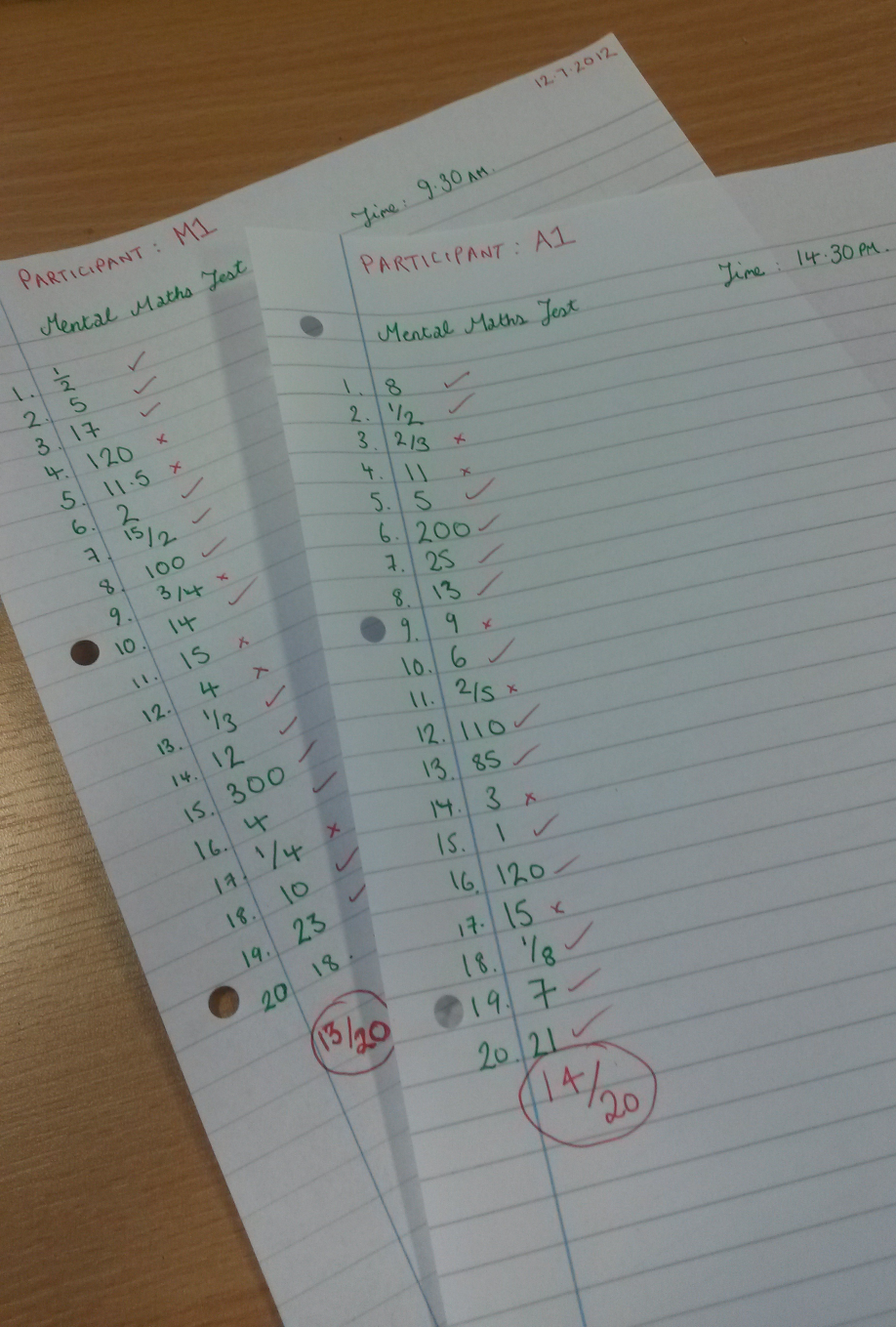
A psychologist wishes to test if people mentally perform differently in the morning compared to the afternoon. He has a group of ten students. They take a mental maths test on the morning and another test on the afternoon with different questions but of the same difficulty. The test scores are shown in the following table.

Morning Scores	Afternoon Scores
13	14
20	19
11	13
9	11
7	10
14	17
12	9
13	16
10	10
17	19

Perform a hypothesis test to see if there is a difference in performance between the morning and afternoon.

Solution

The type of hypothesis test we need to use here is a two sample t-test, since the population standard deviations are unknown and we have a small sample size. We need to use a paired/related t-test, since the morning and afternoon samples are the same participants.

Our hypotheses are:

\begin{align} H_0:& \mu_M = \mu_A\\ H_1:& \mu_M \neq \mu_A\\ \end{align}

where $\mu_M$ and $\mu_A$ are the mean scores of the morning and afternoon tests respectively.

This is a two-tailed test, as we merely wish to know if there is a difference, but have not specified if performance is better in either the afternoon or morning.

First we need to calculate the differences between the scores and mean of these differences. We shall subtract the morning scores from the afternoon scores, and then take the average. We also need to calculate the standard deviation of our two groups.

Morning Scores	Afternoon Scores	Differences
13	14	1
20	19	-1
11	13	2
9	11	2
7	10	3
14	17	3
12	9	-3
13	16	3
10	10	0
17	19	2

The mean of the differences $\bar{d}$ is \[\dfrac{1 - 1 +2 +2 +3 +3 -3 +3 +0 +2}{10} = 1.2.\]

Also note that the mean scores for the morning and afternoon groups are $12.6$ and $13.8$ respectively. We will need to mention these in our conclusion later.

The standard deviation of the difference scores can be calculated using a calculator or in SPSS.

\begin{align} s &= 1.989\\ \end{align}

Now we can calculate our t-statistic, using the formula above. $n = 10$ as there are $10$ participants in each group.

\begin{align} t &= \dfrac{1.2}{~\sqrt{\dfrac{1.989^2}{10}~}~}\\ &= 1.908 \text{ ( 3 d.p.)}.\\ \end{align}

We can compare this to critical t-values on $10 - 1 = 9$ degrees of freedom.

|center

Since $1.908$ is less than the critical value at the $0.05$ level $(1.908<2.262)$, we can conclude that there is no evidence for a difference between afternoon and morning scores. So, mental performance is the same in the afternoon and morning. We accept $H_0$.

We would report out results in the following way:

Test scores were slightly higher in the afternoon $(\bar{X} = 13.8)$ compared to in the morning $(\bar{X}=12.6)$. However, the difference did not support the hypothesis that the tests scores differ in the morning and afternoon at the $0.05$ level of significance $(t = 1.908, \text{df} = 9, p >0.05)$.

Note: df means degrees of freedom.

We can also perform this test in SPSS. To see how, watch the video tutorial below. As you can see, we get the same results as when we performed the test by hand.

Worked Example - Two Sample (unrelated) t-test

You wish to test if the emotionality scores are different between two groups of schoolchildren. One group comes from two-parent families, whereas the other group from one-parent families. You want to know if children from the two-parent families score higher than those from one-parent families. The table of results are below.

' Perform a hypothesis test to test if children from two-parent families score higher than those from one-parent families'

Two Parent Family	One Parent Family
18	5
13	12
12	9
17	11
7	15
11	10
9	12
15
16

Solution

For this example, we will use a two sample t-test, since we not know the population variances and we have sample sizes which are less than $30$.

The null hypothesis is that there is no differences in emotionality scores between the two groups, whereas the alternative hypothesis is that children from two-parent families score higher than those who are from one-parent families.

We have:

\begin{align} H_0:& \bar{x_1} = \bar{x_2}\\ H_1:& \bar{x_1} > \bar{x_2}\\ \end{align}

where $\bar{x_1}$ and $\bar{x_2}$ are the mean scores of the two-parent group and one-parent group respectively.

This is a one tailed test, as we have specified a direction of change.

To calculate our test statistic, we need to calculate the two samples' means and variances and then the pooled standard deviation.

Firstly, for the two-parent group we have,

\begin{align} \bar{x_1} &= \frac{18 + 13 + 12 + 17 + 7 + 11 + 9 + 15 + 16}{9}\\ &= 13.11 \text{ (2 d.p.)}\\ \end{align}

Using our calculator, we find the variance ${s_1}^2 = 13.861$.

For the one-parent group we have, \begin{align} \bar{x_2} &= \frac{5 + 12 + 9 + 11 + 15 + 12 + 10}{7}\\ &= 10.57 \text{ (2 d.p.)}\\ \end{align}

and ${s_2}^2 = 9.619$.

The two-parent group is of size $n_1 = 9$ and the one-parent group is of size $n_2 = 7$.

Now we can calculate $s$ the pooled standard deviation.

\begin{align} s &= \sqrt{\dfrac{(9 - 1) \times 13.861 + (7 - 1) \times 9.619}{9 + 7 - 2}~}\\ &= \sqrt{\dfrac{168.602}{14}~}\\ &= \sqrt{12.043}\\ &= 3.470 \text{ (3 d.p.).}\\ \end{align}

Now we can calculate our test statistic.

\begin{align} t &= \dfrac{13.11 - 10.57}{\sqrt{3.470^2 \times(\frac{1}{9}+\frac{1}{7})}~}\\ &= \dfrac{2.54}{\sqrt{3.058}~}\\ &= 1.452 \text{ (3 d.p.).}\\ \end{align}

We compare it with $t$-values at the $(1 - \alpha)%$ significance levels on $9 + 7 - 2 = 14$ degrees of freedom.

Significance Level	Critical Value
$90\% ~ (0.1)$	$1.345$
$95\% ~ (0.05)$	$1.761$
$99\%~(0.01)$	$2.624$

$1.452<1.761$, so our statistic is not statistically significant at the $5\%$ level. This means we have no evidence against $H_0$ and we can conclude that in this particular study children from two-parent families do not have higher emotionality scores.

In a report we would write:

'It has been found that emotionality scores for the two-parent group $(\bar{X} = 13.1)$ was not significantly higher than the scores for the one-parent group $(\bar{X}=10.9)$ $(t=1.452, \text{df} = 14, p > 0.05, ns)$.'

Note: df means degrees of freedom and ns means not significant.

To see how to perform the test in SPSS watch the video tutorial below.

Test Yourself

Try our Numbas tests on parametric hypothesis tests and two-sample tests.